8 Quantifying life history traits

8.1 Introduction

Capture-recapture models allow the estimation of key demographic parameters such as survival, recruitment, and dispersal. These parameters are central to life history theory, which seeks to explain how organisms allocate limited resources across survival, growth, and reproduction over their lifetime. Life-history traits, such as age at first breeding, breeding frequency, or lifespan, reflect trade-offs shaped by natural selection and environmental constraints.

Capture-recapture data are particularly suited to quantifying such traits in the wild, providing direct estimates that can be compared to theoretical predictions. As introduced in Section 5.5, states and transitions between them – whether disease, developmental, or breeding states – can be incorporated naturally into the HMM framework.

In this chapter, we focus on three examples: cause- and age-specific mortalities, age-specific breeding probabilities, and stopover duration. Together, they illustrate how capture-recapture HMMs can shed light on life-history strategies.

8.2 Assessing age- and cause-specific mortality

8.2.1 Motivation

Cause‐ and age-specific mortalities are key life-history traits, shaping population dynamics and informing management or conservation strategies. Yet in the wild, direct assignment of causes of death is challenging as field observations are often incomplete, and carcass recovery is biased towards certain causes of death or habitats. If we ignore this uncertainty, estimates of mortality rates by cause or age class can be biased, and our understanding of population processes compromised.

The fix is to treat cause of death as a latent state. Following Koons et al. (2014), we model survival and transitions to cause-specific death states jointly within a HMM capture-recapture framework. To do so, we combine data on recaptures of live and recoveries of dead animals. Individuals can either survive to the next occasion or die from one of several competing causes, with probabilities that may depend on age.

Here, we use the case study on roe deer (Capreolus capreolus) in Koons et al. (2014). The authors show that failing to account for uncertain cause assignment underestimated mortality from hunting and overestimated natural mortality, particularly in younger age classes.

Here, we define cause‐specific death states, let survival and cause‐specific mortality depend on age, and keep the rest of the HMM machinery unchanged in NIMBLE.

8.2.2 Model and NIMBLE implementation

For our example, we will use data on roe deer from a population in the enclosed forest of the Territoire d’Etude et d’Expérimentation of Trois Fontaines, in eastern France. Here, we focus on 556 known-age females (marked as fawns), of which 217 were recaptured at least once and 41 were deadly injured during handling, victim of car collisions, or recovered and reported by hunters (human-related mortalities). These data were kindly provided by Marlène Gamelon.

To build up our model, we first define the states and observations:

• States
  - A for alive
  - H for an individual that just died from human causes
  - NH for an individual that just died from a natural (non-human) cause
  - D for an individual that is already dead

• Observations
  - 1 for not seen
  - 2 for captured for the first time or recaptured
  - 3 for killed by human activities and reported

Now we turn to writing our model. We start with the vector of initial states. Individuals enter alive the study with probability 1: \[\begin{matrix} & \\ \mathbf{\delta} = \left ( \vphantom{ \begin{matrix} 12 \end{matrix} } \right . \end{matrix} \hspace{-1.2em} \begin{matrix} z_t=A & z_t=H & z_t=NH & z_t=D \\ \hdashline 1 & 0 & 0 & 0\\ \end{matrix} \hspace{-0.2em} \begin{matrix} & \\ \left . \vphantom{ \begin{matrix} 12 \end{matrix} } \right ) \begin{matrix} \end{matrix} \end{matrix}\]

We proceed with the transition matrix: \[\begin{matrix} & \\ \mathbf{\Gamma} = \left ( \vphantom{ \begin{matrix} 12 \\ 12 \\ 12 \\ 12 \end{matrix} } \right . \end{matrix} \hspace{-1.2em} \begin{matrix} z_t=A & z_t=H & z_t=NH & z_t=D \\ \hdashline 1 - \mu_H - \mu_{NH} & \mu_H & \mu_{NH} & 0\\ 0 & 0 & 0 & 1\\ 0 & 0 & 0 & 1\\ 0 & 0 & 0 & 1 \end{matrix} \hspace{-0.2em} \begin{matrix} & \\ \left . \vphantom{ \begin{matrix} 12 \\ 12 \\ 12 \\ 12 \end{matrix} } \right ) \begin{matrix} z_{t-1}=A \\ z_{t-1}=H \\ z_{t-1}=NH \\ z_{t-1}=D \end{matrix} \end{matrix}\]

where the transition probability from \(A\) at \(t\) to \(H\) at \(t + 1\) is the human-related mortality probability \(\mu_H\) and the transition probability from \(A\) at \(t\) to \(NH\) at \(t + 1\) is the natural mortality probability \(\mu_{NH}\). Because an individual could not return to state \(A\) once dead, we fix these transitions to 0.

Following the paper, adult survival is age-specific: \(\mu_H\) is different for individuals in their first year of life after birth ([0,1[) vs. age 1 onwards, while \(\mu_{NH}\) has two different parameters for ages [0,1[ and [1,2[ then a linear trend with age from age 2 onward. We use a multinomial logit link function to ensure that mortality probabilities are estimated between 0 and 1 and sum up to 1, see Section 5.4.2. In NIMBLE, we code:

# Transition matrix
# Age effects
etaH[i,t] <- (alpha_H_01 * age_lt1[i,t] + alpha_H_ge1 * age_ge1[i,t])

etaNH[i,t] <- (alpha_NH_01 * age_lt1[i,t] +                               # if age is [0,1[
                 alpha_NH_12 * age_1to2[i,t] +                            # if age is [1,2[
                 (beta0_NH + beta1_NH * age_std_mu2[i,t]) * age_ge2[i,t]) # linear trend if age >= 2

# Transitions from A
den[i,t] <- 1 + exp(etaH[i,t]) + exp(etaNH[i,t])  # denominator
gamma[i,t,1,1] <- 1 / den[i,t]                    # stay alive
gamma[i,t,1,2] <- exp(etaH[i,t]) / den[i,t]       # muH
gamma[i,t,1,3] <- exp(etaNH[i,t]) / den[i,t]      # muNH
gamma[i,t,1,4] <- 0                               # always 0

# From H, NH, D (always go to D)
gamma[i,t,2,1] <- 0; gamma[i,t,2,2] <- 0; gamma[i,t,2,3] <- 0; gamma[i,t,2,4] <- 1
gamma[i,t,3,1] <- 0; gamma[i,t,3,2] <- 0; gamma[i,t,3,3] <- 0; gamma[i,t,3,4] <- 1
gamma[i,t,4,1] <- 0; gamma[i,t,4,2] <- 0; gamma[i,t,4,3] <- 0; gamma[i,t,4,4] <- 1

In the code above, age is passed in the data and created as follows:

# Build an N x K age matrix
age <- matrix(0, nrow = nrow(obs_matrix), ncol = K)
for (i in 1:nrow(obs_matrix)) {
  for (t in first[i]:K) {
    age[i, t] <- t - first[i]   # age 0 at first capture
  }
}
# Define age [0,1[ and age >=1
for (i in 1:nrow(obs_matrix)) {
  for (t in first[i]:K) {
    age_val <- age[i, t]
    if (age_val == 0) { # age < 1
      age_lt1[i, t] <- 1
      age_ge1[i, t] <- 0
    } else {            # age >= 1
      age_lt1[i, t] <- 0  
      age_ge1[i, t] <- 1
    }
  }
}
# Define age >1 and age [1,2[
for (i in 1:nrow(obs_matrix)) {
  for (t in first[i]:K) {
    age_val <- age[i, t]
    age_ge2[i, t] <- as.integer(age_val > 1)   # age > 1 or 2 onwards
    age_1to2[i, t] <- as.integer(age_val == 1) # age in [1,2[
  }
}

Last step is the observation matrix: \[\begin{matrix} & \\ \mathbf{\Omega} = \left ( \vphantom{ \begin{matrix} 12 \\ 12 \\ 12 \\ 12 \end{matrix} } \right . \end{matrix} \hspace{-1.2em} \begin{matrix} y_t=1 & y_t=2 & y_t=3\\ \hdashline 1 - p & p & 0 \\ 1 - \lambda & 0 & \lambda\\ 1 & 0 & 0\\ 1 & 0 & 0 \end{matrix} \hspace{-0.2em} \begin{matrix} & \\ \left . \vphantom{ \begin{matrix} 12 \\ 12 \\ 12 \\ 12 \end{matrix} } \right ) \begin{matrix} z_{t}=A \\ z_{t}=H \\ z_{t}=NH \\ z_{t}=D \end{matrix} \end{matrix}\]

where a live individual can be detected with probability \(p\), or not with probability \(1−p\). We include time-dependence and age on \(p\), with a different parameter for 1 year-old individuals vs. individuals older than 1 year of age. In NIMBLE, we write:

pA[i,t] <- p_ageLE1[t] * age_lt1[i,t] + p_ageGT1[t] * age_ge1[i,t]

An individual that just died from human causes can be recovered and reported with probability \(\lambda\), or not with probability \(1-\lambda\). Because tag recovery protocols were constant over the course of the study, the authors considered that parameter to be constant over time and across age classes.

8.2.3 Results and interpretation

The results are given in Figure 8.1. We see senescence in natural mortality from age 2 onwards, as well as well as a slightly higher human-related mortality in the first year of life after birth. These patterns are similar to those obtained by Koons et al. (2014), check out their Figure 4.

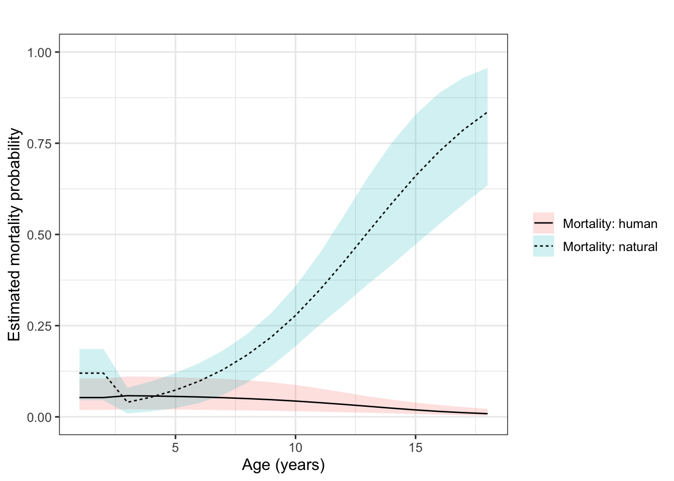
Figure 8.1: Age‐specific mortality probabilities for human‐related (solid line) and natural (dashed line) causes in female roe deer at Trois‐Fontaines, France, from 1985 to 2013. Shaded polygons represent 95% credible intervals.

8.3 Quantifying age-specific breeding

8.3.1 Motivation

Breeding is not a simple yes/no coin flip. Who breeds this year depends on what happened last year. In long-lived mammals, adult survival is high and fairly stable, but breeding probability can differ according to recent reproductive history and with how reliably we detect mothers and their offspring. If we blur these pieces and treat breeding status as perfectly known we risk biasing both survival and breeding estimates.

Couet et al. (2019) give a clear template with female bottlenose dolphins. They show that calf detectability differs by age and a female’s breeding probability depends on the outcome of her previous calf. Rather than assuming states are observed without error, they use a HMM to keep true breeding state hidden, model misclassification/detection explicitly, and tie breeding this year to last year’s outcome. That way, uncertainty about calf presence and age feeds correctly into demographic estimates.

Here, we follow that logic: we define hidden female states (nonbreeder vs. breeder with calf age classes), let detection vary by calf age, and make breeding probability state-dependent on the previous year’s result.

8.3.2 Model and NIMBLE implementation

For our example, we’ll work with data from a population of bottlenose dolphins (Tursiops truncatus) inhabiting the French waters of the Normano-Breton Gulf in the English Channel. We have 106 encounter histories between 2004 and 2016, made of photographs taken from a boat between July and November, which corresponds to the birth peak and the best weather conditions for monitoring. These data were shared by Pauline Couet.

To build up our model, we first define the states and observations:

• States
  - NB for a non-breeding adult female
  - Byoy for a breeding adult female with a young of the year
  - Bc1 for a breeding adult female with a 1‐year‐old calf
  - Bc3 for a breeding adult female with a 3‐year‐old calf
  - Bc2 for a breeding adult female with a 2‐year‐old calf
  - D for a dead female

• Observations
  - 1 for not seen
  - 2 for seen alone
  - 3 for seen with a young of the year
  - 4 for seen with a calf (1 to 3 years old)

Now we turn to writing our model. We start with the vector of initial states: \[ \begin{matrix} & \\ \boldsymbol{\delta} = \left ( \vphantom{ \begin{matrix} 1 \end{matrix} } \right . \end{matrix} \hspace{-1.2em} \begin{matrix} \text{NB} & \text{Byoy} & \text{Bc1} & \text{Bc2} & \text{Bc3} & \text{D} \\ \hdashline \pi_1 & \pi_2 & \pi_3 & \pi_4 & \pi_5 & 0 \end{matrix} \hspace{-0.2em} \begin{matrix} & \\ \left . \vphantom{ \begin{matrix} 1 \end{matrix} } \right ) \end{matrix} \] where \(\displaystyle \pi_5 = 1 - \sum_{j=1}^4\pi_j\).

We proceed with the transition matrix given by Couet et al. (2019): \[ \begin{matrix} & \\ \mathbf{\Gamma} = \left ( \vphantom{ \begin{matrix} 12 \\ 12 \\ 12 \\ 12 \\ 12 \\ 12 \end{matrix} } \right . \end{matrix} \hspace{-1.2em} \begin{matrix} z_t=NB & z_t = Byoy & z_t = Bc1 & z_t = Bc2 & z_t = Bc3 & z_t = D \\ \hdashline \phi_A (1 - \beta_1) & \phi_A \beta_1 & 0 & 0 & 0 & 1 - \phi_A \\ 0 & 0 & \phi_A \phi_Y & \phi_A (1-\phi_Y) & 0 & 1-\phi_A \\ \phi_A (1 - \beta_1) & \phi_A \beta_1 & 0 & 0 & 0 & 1-\phi_A \\ \phi_A (1 - \beta_2) & \phi_A \beta_2 & 0 & 0 & 0 & 1-\phi_A \\ \phi_A (1 - \beta_2) & \phi_A \beta_2 & 0 & 0 & 0 & 1-\phi_A \\ 0 & 0 & 0 & 0 & 0 & 1 \end{matrix} \hspace{-0.2em} \begin{matrix} & \\ \left . \vphantom{ \begin{matrix} 12 \\ 12 \\ 12 \\ 12 \\ 12 \\ 12 \end{matrix} } \right ) \begin{matrix} z_{t-1} = NB \\ z_{t-1} = Byoy \\ z_{t-1} = Bc1 \\ z_{t-1} = Bc2 \\ z_{t-1} = Bc3 \\ z_{t-1} = D \end{matrix} \end{matrix} \]

Rather than attempting to explain the full complexity of this matrix at once, I will follow the authors’ suggestion and break it down into four steps, each corresponding to a biological event in the life cycle of female bottlenose dolphins: (1) female survival \(\mathbf{\Phi_A}\), (2) young survival \(\mathbf{\Phi_Y}\), (3) young aging \(\mathbf{AGING}\), and (4) breeding \(\mathbf{BREED}\), each step being conditional on the previous ones. To do so, we introduce some intermediate states:

• Intermediate states
  - Byoy‐D for a breeding adult female that had lost her young of the year
  - Bc1‐D for a breeding adult female that had lost her 1‐year‐old calf
  - Bc2‐D for a breeding adult female that had lost her 2‐year‐old calf
  - Bc3‐leave Breeding adult female that raised her calf to the age of 3

The four corresponding matrices are given below, starting with the female survival matrix: \[ \begin{matrix} & \\ \mathbf{\Phi_A} = \left ( \vphantom{ \begin{matrix} 12 \\ 12 \\ 12 \\ 12 \\ 12 \\ 12 \end{matrix} } \right . \end{matrix} \hspace{-1.2em} \begin{matrix} \text{NB} & \text{Byoy} & \text{Bc1} & \text{Bc2} & \text{Bc3} & \text{D} \\ \hdashline \phi_A & 0 & 0 & 0 & 0 & 1 - \phi_A \\ 0 & \phi_A & 0 & 0 & 0 & 1 - \phi_A \\ 0 & 0 & \phi_A & 0 & 0 & 1 - \phi_A \\ 0 & 0 & 0 & \phi_A & 0 & 1 - \phi_A \\ 0 & 0 & 0 & 0 & \phi_A & 1 - \phi_A \\ 0 & 0 & 0 & 0 & 0 & 1 \end{matrix} \hspace{-0.2em} \begin{matrix} & \\ \left . \vphantom{ \begin{matrix} 12 \\ 12 \\ 12 \\ 12 \\ 12 \\ 12 \end{matrix} } \right ) \begin{matrix} \text{NB} \\ \text{Byoy} \\ \text{Bc1} \\ \text{Bc2} \\ \text{Bc3} \\ \text{D} \end{matrix} \end{matrix} \]

An adult female survives from \(t\) to \(t+1\) with probability \(\phi_A\) or dies with \(1−\phi_A\). We go on with the young survival matrix: \[ \begin{matrix} & \\ \mathbf{\Phi_Y} = \left ( \vphantom{ \begin{matrix} 12 \\ 12 \\ 12 \\ 12 \\ 12 \\ 12 \end{matrix} } \right . \end{matrix} \hspace{-1.2em} \begin{matrix} \text{NB} & \text{Byoy} & \text{Byoy-D} & \text{Bc1} & \text{Bc1-D} & \text{Bc2} & \text{Bc2-D} & \text{Bc3-leave} & \text{D} \\ \hdashline 1 & 0 & 0 & 0 & 0 & 0 & 0 & 0 & 0 \\ 0 & \phi_{Y} & 1 - \phi_{Y} & 0 & 0 & 0 & 0 & 0 & 0 \\ 0 & 0 & 0 & \phi_{Y} & 1 - \phi_{Y} & 0 & 0 & 0 & 0 \\ 0 & 0 & 0 & 0 & 0 & \phi_{Y} & 1 - \phi_{Y} & 0 & 0 \\ 0 & 0 & 0 & 0 & 0 & 0 & 0 & 1 & 0 \\ 0 & 0 & 0 & 0 & 0 & 0 & 0 & 0 & 1 \end{matrix} \hspace{-0.2em} \begin{matrix} & \\ \left . \vphantom{ \begin{matrix} 12 \\ 12 \\ 12 \\ 12 \\ 12 \\ 12 \end{matrix} } \right ) \begin{matrix} \text{NB} \\ \text{Byoy} \\ \text{Bc1} \\ \text{Bc2} \\ \text{Bc3} \\ \text{D} \end{matrix} \end{matrix} \]

Offspring survive with probability \(\phi_Y\) or die with \(1-\phi_Y\). If the calf survives, the female remains in the same breeding state. If it dies, she moves to an intermediate ‘dead-offspring’ state (BYOY-D, Bc1-D, or Bc2-D) so that later steps can condition on that loss. For 3-year-old calves, mortality cannot be distinguished from emancipation (leaving the mother), so we add an intermediate Bc3-leave state and fix survival to 1 there (this parameter is otherwise unidentifiable). As in the paper, I distinguish young‐of‐the‐year and 1‐year‐old calf survival from 2‐year‐old calf survival. We go on with the young aging matrix: \[ \begin{matrix} & \\ \mathbf{AGING} = \left ( \vphantom{ \begin{matrix} 12 \\ 12 \\ 12 \\ 12 \\ 12 \\ 12 \\ 12 \\ 12 \\ 12 \end{matrix} } \right . \end{matrix} \hspace{-1.2em} \begin{matrix} \text{NB} & \text{Byoy} & \text{Byoy-D} & \text{Bc1} & \text{Bc1-D} & \text{Bc2} & \text{Bc2-D} & \text{Bc3-leave} & \text{D} \\ \hdashline 1 & 0 & 0 & 0 & 0 & 0 & 0 & 0 & 0 \\ 0 & 1 & 0 & 0 & 0 & 0 & 0 & 0 & 0 \\ 0 & 0 & 1 & 0 & 0 & 0 & 0 & 0 & 0 \\ 0 & 0 & 0 & 0 & 1 & 0 & 0 & 0 & 0 \\ 0 & 0 & 0 & 0 & 1 & 0 & 0 & 0 & 0 \\ 0 & 0 & 0 & 0 & 0 & 0 & 1 & 0 & 0 \\ 0 & 0 & 0 & 0 & 0 & 0 & 1 & 0 & 0 \\ 0 & 0 & 0 & 0 & 0 & 0 & 0 & 1 & 0 \\ 0 & 0 & 0 & 0 & 0 & 0 & 0 & 0 & 1 \end{matrix} \hspace{-0.2em} \begin{matrix} & \\ \left . \vphantom{ \begin{matrix} 12 \\ 12 \\ 12 \\ 12 \\ 12 \\ 12 \\ 12 \\ 12 \\ 12 \end{matrix} } \right ) \begin{matrix} \text{NB} \\ \text{Byoy} \\ \text{Byoy-D} \\ \text{Bc1} \\ \text{Bc1-D} \\ \text{Bc2} \\ \text{Bc2-D} \\ \text{Bc3-leave} \\ \text{D} \end{matrix} \end{matrix} \] The progression of calf age classes between \(t\) and \(t+1\) is deterministic, all relevant age-advancing transitions are set to 1, and there are no parameters estimated in this matrix. Last, here is the breeding matrix: \[ \begin{matrix} & \\ \mathbf{BREED} = \left ( \vphantom{ \begin{matrix} 12 \\ 12 \\ 12 \\ 12 \\ 12 \\ 12 \\ 12 \\ 12 \\ 12 \end{matrix} } \right . \end{matrix} \hspace{-1.2em} \begin{matrix} \text{NB} & \text{Byoy} & \text{Bc1} & \text{Bc2} & \text{Bc3} & \text{D} \\ \hdashline 1 - \beta_1 & \beta_1 & 0 & 0 & 0 & 0 \\ 0 & 0 & 1 & 0 & 0 & 0 \\ 0 & 0 & 0 & 1 & 0 & 0 \\ 0 & 0 & 0 & 0 & 1 & 0 \\ 1 - \beta_1 & \beta_1 & 0 & 0 & 0 & 0 \\ 1 - \beta_1 & \beta_1 & 0 & 0 & 0 & 0 \\ 1 - \beta_2 & \beta_2 & 0 & 0 & 0 & 0 \\ 1 - \beta_2 & \beta_2 & 0 & 0 & 0 & 0 \\ 0 & 0 & 0 & 0 & 0 & 1 \end{matrix} \hspace{-0.2em} \begin{matrix} & \\ \left . \vphantom{ \begin{matrix} 12 \\ 12 \\ 12 \\ 12 \\ 12 \\ 12 \\ 12 \\ 12 \\ 12 \end{matrix} } \right ) \begin{matrix} \text{NB} \\ \text{Byoy} \\ \text{Bc1} \\ \text{Bc2} \\ \text{Byoy-D} \\ \text{Bc1-D} \\ \text{Bc2-D} \\ \text{Bc3-leave} \\ \text{D} \end{matrix} \end{matrix} \]

Breeding at \(t+1\) occurs with probability \(\beta\) (otherwise \(1−\beta\)). Breeding can depend on the female’s state, namely non-breeding females and females that had just lost their young of the year or 1‐year‐old calf (\(\beta_1\)) vs. females that had lost their 2‐year‐old calf or raised it until the age of 3 (\(\beta_2\)).

Overall, the transition matrix is the product of all four matrices. In NIMBLE, we could code directly the full matrix, but I take this opportunity to illustrate how to code the splitting in several ecological processes:

# Transition matrix

# PHIA is 6x6
for (i in 1:5) {
  PHIA[i, i] <- adultsurvival
  PHIA[i, 6] <- 1 - adultsurvival
}
PHIA[6, 6] <- 1

# PHIY is 6x9
# Row 1: NB stays NB
PHIY[1, 1] <- 1
# Row 2: Byoy
PHIY[2, 2] <- youngsurvival[1]        # YOY survives → becomes Bc1
PHIY[2, 3] <- 1 - youngsurvival[1]    # YOY dies     → becomes Byoy-D
# Row 3: Bc1
PHIY[3, 4] <- youngsurvival[1]        # 1-year-old survives → Bc2
PHIY[3, 5] <- 1 - youngsurvival[1]    # dies → Bc1-D
# Row 4: Bc2
PHIY[4, 6] <- youngsurvival[2]        # 2-year-old survives → Bc3-L (emancipation)
PHIY[4, 7] <- 1 - youngsurvival[2]    # dies → Bc2-D
# Row 5: Bc3 always emancipates
PHIY[5, 8] <- 1
# Row 6: dead female stays dead
PHIY[6, 9] <- 1

# AGING is 9x9
AGING[1, 1] <- 1   # NB → NB
AGING[2, 2] <- 1   # Byoy → Bc1
AGING[3, 5] <- 1   # Byoy-D → Byoy-D
AGING[4, 3] <- 1   # Bc1 → Bc2
AGING[5, 6] <- 1   # Bc1-D → Bc1-D
AGING[6, 4] <- 1   # Bc2 → Bc3
AGING[7, 7] <- 1   # Bc2-D → Bc2-D
AGING[8, 8] <- 1   # Bc3-L → Bc3-L
AGING[9, 9] <- 1   # D → D

# BREED is 9x6
# Row 1: NB → Byoy or NB
BREED[1, 2] <- beta[1]
BREED[1, 1] <- 1 - beta[1]
# Row 2: Bc1 → Bc1
BREED[2, 3] <- 1
# Row 3: Bc2 → Bc2
BREED[3, 4] <- 1
# Row 4: Bc3 → Bc3
BREED[4, 5] <- 1
# Row 5: Byoy-D → Byoy or NB
BREED[5, 2] <- beta[1]
BREED[5, 1] <- 1 - beta[1]
# Row 6: Bc1-D → Byoy or NB
BREED[6, 2] <- beta[1]
BREED[6, 1] <- 1 - beta[1]
# Row 7: Bc2-D → Byoy or NB
BREED[7, 2] <- beta[2]
BREED[7, 1] <- 1 - beta[2]
# Row 8: Bc3-L → Byoy or NB
BREED[8, 2] <- beta[2]
BREED[8, 1] <- 1 - beta[2]
# Row 9: D → D
BREED[9, 6] <- 1

gamma[1:6,1:6] <- PHIA[1:6,1:6] %*% PHIY[1:6,1:9] %*% AGING[1:9,1:9] %*% BREED[1:9,1:6]

Last step is the observation matrix that we can also split in two steps, given these intermediate observations:

• ND: for not detected
  
• DNB: for a non-breeding female detected at time \(t\)
  
• DByoy: for a breeding female with a young of the year detected at time \(t\)
  
• DBc: for a breeding female with a 1-year-old calf detected at time \(t\)
  
• DBc2: for a breeding female with a 2-year-old calf detected at time \(t\)
  
• DBc3: for a breeding female with a 3-year-old calf detected at time \(t\)

First, the detection step: \[ \begin{matrix} & \\ \mathbf{DETECTION} = \left ( \vphantom{ \begin{matrix} 12 \\ 12 \\ 12 \\ 12 \\ 12 \\ 12 \end{matrix} } \right . \end{matrix} \hspace{-1.2em} \begin{matrix} \text{ND} & \text{DNB} & \text{DByoy} & \text{DBc} & \text{DBc2} & \text{DBc3} \\ \hdashline 1 - p_1 & p_1 & 0 & 0 & 0 & 0 \\ 1 - p_2 & 0 & p_2 & 0 & 0 & 0 \\ 1 - p_2 & 0 & 0 & p_2 & 0 & 0 \\ 1 - p_1 & 0 & 0 & 0 & p_1 & 0 \\ 1 - p_1 & 0 & 0 & 0 & p_1 & 0 \\ 1 & 0 & 0 & 0 & 0 & 0 \end{matrix} \hspace{-0.2em} \begin{matrix} & \\ \left . \vphantom{ \begin{matrix} 12 \\ 12 \\ 12 \\ 12 \\ 12 \\ 12 \end{matrix} } \right ) \begin{matrix} \text{NB} \\ \text{Byoy} \\ \text{Bc1} \\ \text{Bc2} \\ \text{Bc3} \\ \text{D} \end{matrix} \end{matrix} \]

which contains the probability \(p\) of detecting the female given her latent state at \(t\): \(p_2\) is for females with a young of the year or a 1‐year‐old calf and \(p_1\) for non-breeding females or those with an older calf. Then the observation matrix: \[ \begin{matrix} & \\ \mathbf{OBS} = \left ( \vphantom{ \begin{matrix} 12 \\ 12 \\ 12 \\ 12 \\ 12 \\ 12 \end{matrix} } \right . \end{matrix} \hspace{-1.2em} \begin{matrix} 1 & 2 & 3 & 4 \\ \hdashline 1 & 0 & 0 & 0 \\ 0 & 1 & 0 & 0 \\ 0 & 1 - q_1 & q_1 & 0 \\ 0 & 1 - q_2 & 0 & q_2 \\ 0 & 1 - q_2 & 0 & q_2 \\ 0 & 1 - q_2 & 0 & q_2 \end{matrix} \hspace{-0.2em} \begin{matrix} & \\ \left . \vphantom{ \begin{matrix} 12 \\ 12 \\ 12 \\ 12 \\ 12 \\ 12 \end{matrix} } \right ) \begin{matrix} \text{ND} \\ \text{DNB} \\ \text{DByoy} \\ \text{DBc} \\ \text{DBc2} \\ \text{DBc3} \end{matrix} \end{matrix} \]

where, conditional on being in a breeding state, there is a probability \(q\) that a calf is seen vs. not seen. Calf age is not identifiable from photographs, so observations are seen or not seen, but \(q\) may still vary by calf age (here young of the year vs. older). This is coded in NIMBLE as follows:

# Observation matrix

# Detection probabilities
DETECTION[1, 1] <- 1 - p[1]     # NB not detected
DETECTION[1, 2] <- p[1]         # NB detected
DETECTION[2, 1] <- 1 - p[2]
DETECTION[2, 3] <- p[2]        # Byoy detected
DETECTION[3, 1] <- 1 - p[2]
DETECTION[3, 4] <- p[2]         # Bc1 detected
DETECTION[4, 1] <- 1 - p[1]
DETECTION[4, 5] <- p[1]         # Bc2 detected
DETECTION[5, 1] <- 1 - p[1]
DETECTION[5, 6] <- p[1]         # Bc3 detected
DETECTION[6, 1] <- 1           # Dead never detected

# OBS is 6x4
# Not detected → not sighted
OBS[1, 1] <- 1
# Detected NB → alone
OBS[2, 2] <- 1
# Detected Byoy → YOY visible or not
OBS[3, 2] <- 1 - q[1]    # alone
OBS[3, 3] <- q[1]        # with YOY
# Detected Bc1 → calf visible or not
OBS[4, 2] <- 1 - q[2]
OBS[4, 4] <- q[2]
# Detected Bc2
OBS[5, 2] <- 1 - q[2]
OBS[5, 4] <- q[2]
# Detected Bc3
OBS[6, 2] <- 1 - q[2]
OBS[6, 4] <- q[2]

omega[1:6,1:4] <- DETECTION[1:6,1:6] %*% OBS[1:6,1:4]

8.3.3 Results and interpretation

The raw results are:

##                  mean   sd 2.5%  50% 97.5% Rhat n.eff
## adultsurvival    0.96 0.01 0.94 0.96  0.98 1.00  2069
## beta[1]          0.35 0.04 0.28 0.35  0.45 1.03   656
## beta[2]          0.57 0.10 0.39 0.57  0.78 1.00  1009
## p[1]             0.63 0.03 0.58 0.63  0.69 1.00  1764
## p[2]             0.79 0.03 0.72 0.79  0.86 1.00  1123
## pi[1]            0.49 0.06 0.37 0.49  0.60 1.01  2743
## pi[2]            0.26 0.05 0.17 0.26  0.37 1.00  3412
## pi[3]            0.08 0.03 0.03 0.08  0.16 1.00  2225
## pi[4]            0.14 0.04 0.07 0.14  0.23 1.00  1931
## pi[5]            0.03 0.03 0.00 0.02  0.10 1.02  1315
## q[1]             0.59 0.05 0.49 0.59  0.69 1.01  1091
## q[2]             0.80 0.05 0.70 0.80  0.89 1.01   818
## youngsurvival[1] 0.63 0.05 0.55 0.63  0.73 1.00   808
## youngsurvival[2] 0.69 0.08 0.53 0.69  0.83 1.00  1702

which we can re-arrange as in Table 8.1 to compare them to the estimates obtained by Couet et al. (2019):

Table 8.1: Age-specific estimates of breeding probabilities. Comparison of our NIMBLE estimates with Couet et al. (2019). ‘NR’ denotes quantities not reported in the paper. ‘NB’ is for non-breeding and ‘yoy’ for young-of-the-year. Adult female detection on the paper side is a rough time-average read by eye from the authors’ Figure 3 (2005–2016).

Parameter	NIMBLE	Couet
Adult female survival	0.96 (0.94–0.98)	0.97 (0.96-0.98)
Calf observation, yoy	0.59 (0.49–0.69)	0.58 (0.46-0.68)
Calf observation, 1-3y	0.80 (0.70–0.89)	0.79 (0.59-0.90)
Calf survival (yoy)	0.63 (0.55–0.73)	0.66 (0.50-0.78)
Calf survival (1y)	0.69 (0.53–0.83)	0.45 (0.29-0.61)
Female detection: NB or calf 2-3y	0.63 (0.58–0.69)	≈0.47
Female detection: yoy or 1-year calf	0.79 (0.72–0.86)	≈0.61
Initial state NB	0.49 (0.37–0.60)	NR
Initial state Byoy	0.26 (0.17–0.37)	NR
Initial state Bc1	0.08 (0.03–0.16)	NR
Initial state Bc2	0.14 (0.07–0.23)	NR
Initial state Bc3	0.03 (0.00–0.10)	NR

Our NIMBLE estimates track the published values closely. Calf survival shows some discrepancies, but credible and confidence intervals overlap, so I would not worry too much. Note also that our model differs slightly: we held adult female detection constant in time, whereas the paper models it as time‐dependent.

Offspring are often missed even when a female is breeding, especially young of the year, which are harder to see than older calves. Offspring detection is well below 1. Adult detection also depends on the female’s state: females with a young of the year or 1-year calf are more detectable than non-breeders or those with older calves.

Adult female survival is high. Calf survival ranks young-of-the-year ≥ 1-year. Breeding probability depends on recent history: it’s lower after non-breeding or losing a young-of-the-year/1-year calf, and higher after losing a 2-year calf or successfully raising a calf to age 3.

8.4 Estimating stopover duration

8.4.1 Motivation

Stopover is not just a logistical pause; it’s a stage-specific timing trait in a migratory life cycle. Like age at first reproduction or length of a breeding attempt, the duration of stopover shapes exposure to predators, energy balance, and downstream reproductive timing. Two core questions in migration ecology are: (1) how long individuals stop over, and (2) whether groups differ in their stopover behaviour. Treating stopover as a life-history trait puts those questions center stage.

The catch is that arrivals and departures are hidden and detection is imperfect. If we only look at when individuals are seen, we bias both the entry curve and the distribution of stay lengths. As reviewed in Guérin et al. (2017), a HMM fixes this by keeping states hidden and observations separate: for example, we may use three latent states: not yet arrived, arrived (present), departed; and let two transition probabilities drive dynamics: recruitment (from not yet arrived to arrived) and staying (from arrived to arrived). Detection operates only in state arrived. This so-called time-effect parameterization assumes staying depends on calendar date, not time since arrival, which is often the right first step.

With this setup we can estimate daily entry and staying probabilities, derive expected stopover duration for an arrival date, and test for group differences in behaviour.

8.4.2 Model and NIMBLE implementation

We illustrate the model with marbled newts (Triturus marmoratus) monitored in 2013 at a permanent pond near Vigneux-de-Bretagne (Loire-Atlantique, western France). Intensive capture-recapture yielded 713 PIT-tagged newts (412 males, 301 females). Captures within the same week were pooled to create 12 equally spaced occasions (11 weekly samples plus a leading ‘empty’ occasion), so all individuals start in the ‘not yet arrived’ state. These data were shared by Sandra Guérin.

To build up our model, we first define the states and observations:

• States
  - NYA for not yet arrived in the pond
  - ARR for arrived in the pond
  - DEP departed from the pond

• Observations
  - 1 for not captured
  - 2 for captured

Now we turn to writing our model. We start with the vector of initial states. At the start of the study, everyone is in \(NYA\), so the initial state vector is: \[ \begin{matrix} & \\ \boldsymbol{\delta} = \left ( \vphantom{ \begin{matrix} 1 \end{matrix} } \right . \end{matrix} \hspace{-1.2em} \begin{matrix} \text{NYA} & \text{ARR} & \text{DEP} \\ \hdashline 1 & 0 & 0 \end{matrix} \hspace{-0.2em} \begin{matrix} & \\ \left . \vphantom{ \begin{matrix} 1 \end{matrix} } \right ) \end{matrix} \]

We proceed with the transition matrix, which is governed by two processes: recruitment \(r\) is the probability that an individual in \(NYA\) enters the pond and staying \(s\) is the probability that an individual in \(ARR\) remains in the pond. State \(DEP\) is absorbing. We have: \[\begin{matrix} & \\ \mathbf{\Gamma} = \left ( \vphantom{ \begin{matrix} 12 \\ 12 \\ 12 \end{matrix} } \right . \end{matrix} \hspace{-1.2em} \begin{matrix} z_t=NYA & z_t=ARR & z_t=DEP \\ \hdashline 1 - r & r & 0 \\ 0 & s & 1 - s \\ 0 & 0 & 1 \end{matrix} \hspace{-0.2em} \begin{matrix} & \\ \left . \vphantom{ \begin{matrix} 12 \\ 12 \\ 12 \end{matrix} } \right ) \begin{matrix} z_{t-1}=NYA \\ z_{t-1}=ARR \\ z_{t-1}=DEP \end{matrix} \end{matrix}\]

We make both parameters \(r\) and \(s\) sex and time-dependent, which we code in NIMBLE:

for (j in 1:(K-1)){
  logit(r[1,j]) <- beta[1,1] + beta[1,2] * (j-4.5)/2.45 # prior probability of arriving in the pond / 1 = female
  logit(r[2,j]) <- beta[2,1] + beta[2,2] * (j-4.5)/2.45 # prior probability of arriving in the pond / 2 = male
  s[1,j] ~ dunif(0, 1) # prior retention probability (staying) / 1 = female
  s[2,j] ~ dunif(0, 1) # prior retention probability (staying) / 2 = male
}
for (i in 1:N){
  for (j in 1:(K-1)){
    gamma[1,1,i,j] <- 1 - r[sex[i],j] 
    gamma[1,2,i,j] <- r[sex[i],j] 
    gamma[1,3,i,j] <- 0 
    gamma[2,1,i,j] <- 0
    gamma[2,2,i,j] <- s[sex[i],j]
    gamma[2,3,i,j] <- 1 - s[sex[i],j]
    gamma[3,1,i,j] <- 0 
    gamma[3,2,i,j] <- 0 
    gamma[3,3,i,j] <- 1
  }
}

Graphically, this corresponds to:

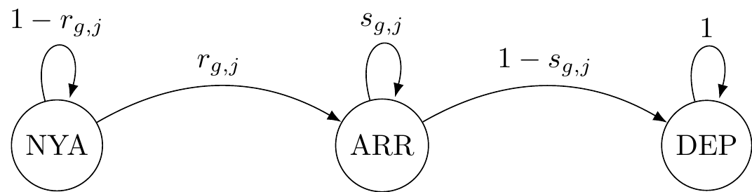
Last step is the observation matrix: \[\begin{matrix} & \\ \mathbf{\Omega} = \left ( \vphantom{ \begin{matrix} 12 \\ 12 \\ 12 \end{matrix} } \right . \end{matrix} \hspace{-1.2em} \begin{matrix} y_t=1 & y_t=2 \\ \hdashline 1 & 0 \\ 1-p & p \\ 1 & 0 \end{matrix} \hspace{-0.2em} \begin{matrix} & \\ \left . \vphantom{ \begin{matrix} 12 \\ 12 \\ 12 \end{matrix} } \right ) \begin{matrix} z_{t}=NYA \\ z_{t}=ARR \\ z_{t}=DEP \end{matrix} \end{matrix}\]

where only individuals in state \(ARR\) are observable with probability \(p\).

The likelihood and priors are handled as usual.

Using MCMC draws from the posterior distribution of the staying probability \(s\), we can calculate the expected stopover duration \(\mathbb{E}[D]\) which is the number of occasions present after arrival. With constant \(s\), this is given by: \[ \mathbb{E}[D] \;=\; \frac{1}{\,1 - s\,}. \]

Why is that? Because the length of stay (counting the arrival occasion) is geometric. After arriving, you are present this week with probability 1 (that’s 1 week). You are still present next week with probability \(s\). You are still present the week after with probability \(s^2\). And so on. So the expected number of occasions present is the sum of those probabilities:

\[ \mathbb{E}[D] \;=\; 1+s+s^2+\cdots \;=\; \frac{1}{\,1 - s\,}. \]

When \(s\) varies with date, the ‘length of stay’ after arrival is no longer geometric with a single parameter, it’s a non-homogeneous geometric process with week-specific stay probabilities \(s_t\). If an individual arrives on date \(\tau\), the chance it is still present \(k\) occasions later is the product of the stay probabilities along that run:

\[ Pr(D > k \mid \text{arrive at } \tau) \;=\; \prod_{j=0}^{k-1} s_{\tau + j}. \]

Therefore, the expected number of occasions present (counting the arrival occasion) is the sum of those tail probabilities: \[ \mathbb{E}[D \mid \text{arrive at } \tau] \;=\; \sum_{k=0}^{\infty} \prod_{j=0}^{k-1} s_{\tau + j}. \]

with the empty product for \(k=0\) equal to 1, or in other words the sum of the probabilities of ‘surviving’ each additional week in \(ARR\) under the calendar-date effects.

8.4.3 Results and interpretation

Our NIMBLE estimates match pretty closely those obtained by Guérin et al. (2017), check out their Figure 2.

Early in the season, females arrive first: during the first three capture occasions their arrival probability exceeds that of males (Figure 8.2). By occasion 7, essentially all individuals have entered the pond.

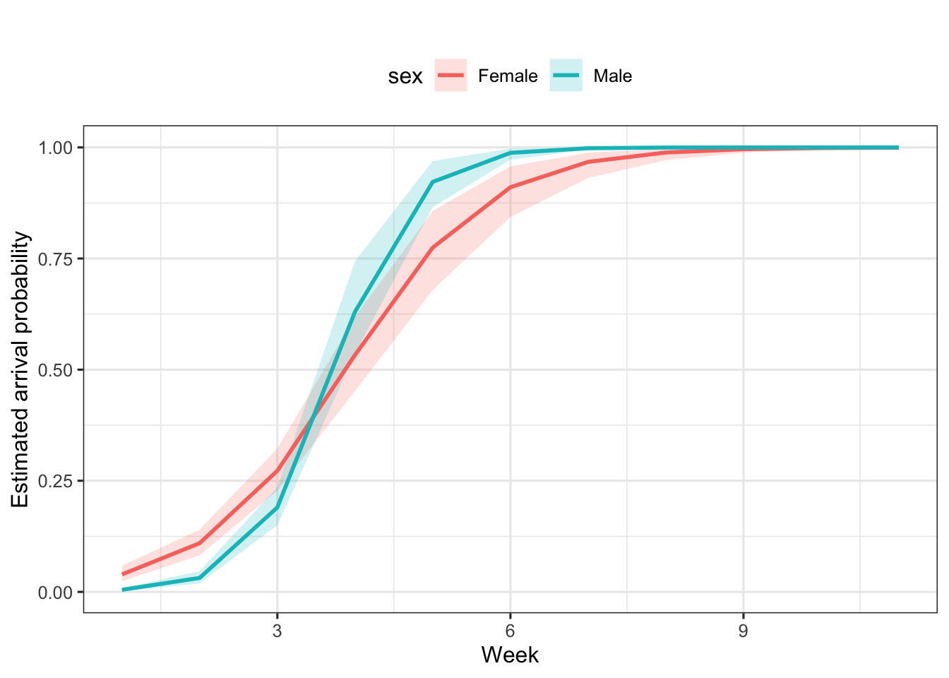
Figure 8.2: Arrival probability by sex and week. Means and 95% credible intervals (shaded areas) are provided.

Females show longer stopovers than males for most of the season; near the end, the pattern reverses (Figure 8.3). Individuals arriving early in the breeding season stay longer than those arriving later.

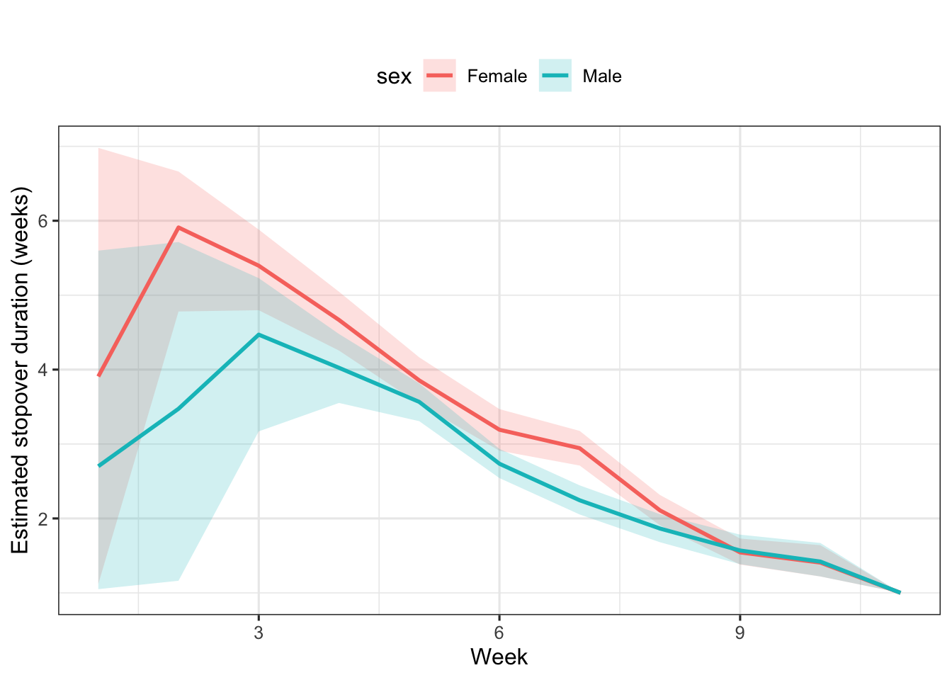
Figure 8.3: Stopover duration by sex and arrival week. Means and 95% credible intervals (shaded areas) are provided.