3 Hidden Markov models

3.1 Introduction

In this third chapter, you will learn the basics on Markov models and how to fit them to longitudinal data using NIMBLE. In real life however, individuals may go undetected and their status be unknown. You will also learn how to manipulate the extension of Markov models to hidden states, so-called hidden Markov models.

3.2 Longitudinal data

Let’s get back to our survival example, and denote \(z_i\) the state of individual \(i\) with \(z_i = 1\) if alive and \(z_i = 0\) if dead. We have a total of \(z = \displaystyle{\sum_{i=1}^{n}{z_i}}\) survivors out of \(n\) released animals with winter survival probability \(\phi\). Our model so far is a combination of a binomial likelihood and a Beta prior with parameters 1 and 1, which is also a uniform distribution between 0 and 1. It can be written as:

\[\begin{align*} z &\sim \text{Binomial}(n, \phi) &\text{[likelihood]} \\ \phi &\sim \text{Beta}(1, 1) &\text{[prior for }\phi \text{]} \\ \end{align*}\]

Because the binomial distribution is just a sum of independent Bernoulli outcomes, you can rewrite this model as:

\[\begin{align*} z_i &\sim \text{Bernoulli}(\phi), \; i = 1, \ldots, N &\text{[likelihood]} \\ \phi &\sim \text{Beta}(1, 1) &\text{[prior for }\phi \text{]} \\ \end{align*}\]

It is like flipping a coin for each individual and get a survivor with probability \(\phi\).

In this set up, we consider a single winter. But for many species, we need to collect data on the long term to get a representative estimate of survival. Therefore what if we had say \(T = 5\) winters?

Let us denote \(z_{i,t} = 1\) if individual \(i\) alive at winter \(t\), and \(z_{i,t} = 2\) if dead. Then longitudinal data look like in the table below. Each row is an individual \(i\), and columns are for winters \(t\), or sampling occasions. Variable \(z\) is indexed by both \(i\) and \(t\), and takes value 1 if individual \(i\) is alive in winter \(t\), and 2 otherwise.

## # A tibble: 57 × 6
##       id `winter 1` `winter 2` `winter 3` `winter 4`
##    <int>      <int>      <int>      <int>      <int>
##  1     1          1          1          1          1
##  2     2          1          1          1          1
##  3     3          1          1          1          1
##  4     4          1          1          1          1
##  5     5          1          1          1          1
##  6     6          1          1          2          2
##  7     7          1          1          1          1
##  8     8          1          2          2          2
##  9     9          1          1          1          1
## 10    10          1          2          2          2
## # ℹ 47 more rows
## # ℹ 1 more variable: `winter 5` <int>

3.3 A Markov model for longitudinal data

Let’s think of a model for these data. The objective remains the same, estimating survival. To build this model, we’ll make assumptions, go through its components and write down its likelihood. Note that we have already encountered Markov models in Section 1.5.2.

3.3.1 Assumptions

First, we assume that the state of an animal in a given winter, alive or dead, is only dependent on its state the winter before. In other words, the future depends only on the present, not the past. This is a Markov process.

Second, if an animal is alive in a given winter, the probability it survives to the next winter is \(\phi\). The probability it dies is \(1 - \phi\).

Third, if an animal is dead a winter, it remains dead, unless you believe in zombies.

Our Markov process can be represented this way:

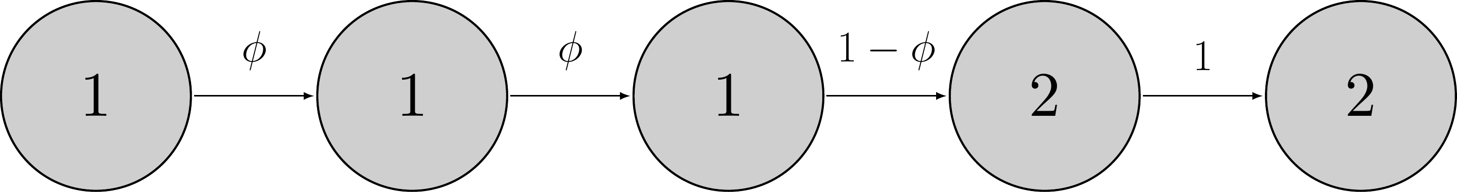
An example of this Markov process is, for example:

Here the animal remains alive over the first two time intervals \((z_{i,1} = z_{i,2} = z_{i,3} = 1)\) with probability \(\phi\) until it dies over the fourth time interval \((z_{i,4} = 2)\) with probability \(1-\phi\) then remains dead from then onwards \((z_{i,5} = 2)\) with probability 1.

3.3.2 Transition matrix

You might have figured it out already (if not, not a problem), the core of our Markov process is made of transition probabilities between states alive and dead. For example, the probability of transitioning from state alive at \(t-1\) to state alive at \(t\) is \(\Pr(z_{i,t} = 1 | z_{i,t-1} = 1) = \gamma_{1,1}\). It is the survival probability \(\phi\). The probability of dying over the interval \((t-1, t)\) is \(\Pr(z_{i,t} = 2 | z_{i,t-1} = 1) = \gamma_{1,2} = 1 - \phi\). Now if an animal is dead at \(t-1\), then \(\Pr(z_t = 1 | z_{t-1} = 2) = 0\) and \(\Pr(z_{i,t} = 2 | z_{i,t-1} = 2) = 1\).

We can gather these probabilities of transition between states from one occasion to the next in a matrix, say \(\mathbf{\Gamma}\), which we will call the transition matrix:

\[\begin{align*} \mathbf{\Gamma} = \left(\begin{array}{cc} \gamma_{1,1} & \gamma_{1,2}\\ \gamma_{2,1} & \gamma_{2,2} \end{array}\right) = \left(\begin{array}{cc} \phi & 1 - \phi\\ 0 & 1 \end{array}\right) \end{align*}\]

To try and remember that the states at \(t-1\) are in rows, and the states at \(t\) are in columns, I will often write:

\[\begin{matrix} & \\ \mathbf{\Gamma} = \left ( \vphantom{ \begin{matrix} 12 \\ 12 \end{matrix} } \right . \end{matrix} \hspace{-1.2em} \begin{matrix} z_t=1 & z_t=2 \\ \hdashline \phi & 1-\phi \\ 0 & 1 \end{matrix} \hspace{-0.2em} \begin{matrix} & \\ \left . \vphantom{ \begin{matrix} 12 \\ 12 \end{matrix} } \right ) \begin{matrix} z_{t-1}=1 \; \mbox{(alive)} \\ z_{t-1}=2 \; \mbox{(dead)} \end{matrix} \end{matrix}\]

Take the time you need to navigate through this matrix, and get familiar with it. For example, you may start alive at \(t\) (first row) then end up dead at \(t+1\) (first column) with probability \(1-\phi\).

3.3.3 Initial states

A Markov process has to start somewhere. We need the probabilities of initial states, i.e. the states of an individual at \(t = 1\). We will gather the probability of being in each state (alive or 1 and dead or 2) in the first winter in a vector. We will use \(\mathbf{\delta} = \left(\Pr(z_{i,1} = 1), \Pr(z_{i,1} = 2)\right)\). For simplicity, we will assume that all individuals are marked and released in the first winter, hence alive when first captured, which means that they are all in state alive or 1 for sure. Therefore we have \(\mathbf{\delta} = \left(1, 0\right)\).

3.3.4 Likelihood

Now that we have built a Markov model, we need its likelihood to apply the Bayes theorem. The likelihood is the probability of the data, given the model. Here the data are the \(z\), therefore we need \(\Pr(\mathbf{z}) = \Pr(z_1, z_2, \ldots, z_{T-2}, z_{T-1}, z_T)\).

We’re gonna work backward, starting from the last sampling occasion. Using conditional probabilities, the likelihood can be written as the product of the probability of \(z_T\) i.e. you’re alive or not on the last occasion given your past history, that is the states at previous occasions, times the probability of your past history:

\[\begin{align*} \Pr(\mathbf{z}) &= \Pr(z_T, z_{T-1}, z_{T-2}, \ldots, z_1) \color{white}{\Pr(z_{T-1}, z_{T-2},\ldots, z_1) \Pr(z_{T-2}, \ldots, z_1)}\\ &= \color{blue}{\Pr(z_T | z_{T-1}, z_{T-2},\ldots, z_1) \Pr(z_{T-1}, z_{T-2},\ldots, z_1)} \\ \end{align*}\]

Then because we have a Markov model, we’re memory less, that is the probabilty of next state, here \(z_T\), depends only on the current state, that is \(z_{T-1}\), and not the previous states:

\[\begin{align*} \Pr(\mathbf{z}) &= \Pr(z_T, z_{T-1}, z_{T-2}, \ldots, z_1) \color{white}{\Pr(z_{T-1}, z_{T-2},\ldots, z_1) \Pr(z_{T-2}, \ldots, z_1)}\\ &= \Pr(z_T | z_{T-1}, z_{T-2},\ldots, z_1) \Pr(z_{T-1}, z_{T-2},\ldots, z_1) \\ &= \color{blue}{\Pr(z_T | z_{T-1})} \Pr(z_{T-1}, z_{T-2},\ldots, z_1) \\ \end{align*}\]

You can apply the same reasoning to \(T-1\). First use conditional probabilities:

\[\begin{align*} \Pr(\mathbf{z}) &= \Pr(z_T, z_{T-1}, z_{T-2}, \ldots, z_1) \color{white}{\Pr(z_{T-1}, z_{T-2},\ldots, z_1) \Pr(z_{T-2}, \ldots, z_1)}\\ &= \Pr(z_T | z_{T-1}, z_{T-2},\ldots, z_1) \Pr(z_{T-1}, z_{T-2},\ldots, z_1) \\ &= \Pr(z_T | z_{T-1}) \Pr(z_{T-1}, z_{T-2},\ldots, z_1) \\ &= \Pr(z_T | z_{T-1}) \color{blue}{\Pr(z_{T-1} | z_{T-2}, \ldots, z_1) \Pr(z_{T-2}, \ldots, z_1)}\\ \end{align*}\]

Then apply the Markovian property:

\[\begin{align*} \Pr(\mathbf{z}) &= \Pr(z_T, z_{T-1}, z_{T-2}, \ldots, z_1) \color{white}{\Pr(z_{T-1}, z_{T-2},\ldots, z_1) \Pr(z_{T-2}, \ldots, z_1)}\\ &= \Pr(z_T | z_{T-1}, z_{T-2},\ldots, z_1) \Pr(z_{T-1}, z_{T-2},\ldots, z_1) \\ &= \Pr(z_T | z_{T-1}) \Pr(z_{T-1}, z_{T-2},\ldots, z_1) \\ &= \Pr(z_T | z_{T-1}) \Pr(z_{T-1} | z_{T-2}, \ldots, z_1) \Pr(z_{T-2}, \ldots, z_1)\\ &= \Pr(z_T | z_{T-1}) \color{blue}{\Pr(z_{T-1} | z_{T-2})} \Pr(z_{T-2}, \ldots, z_1)\\ \end{align*}\]

And so on up to \(z_2\). You end up with this expression for the likelihood:

\[\begin{align*} \Pr(\mathbf{z}) &= \Pr(z_T, z_{T-1}, z_{T-2}, \ldots, z_1) \color{white}{\Pr(z_{T-1}, z_{T-2},\ldots, z_1) \Pr(z_{T-2}, \ldots, z_1)}\\ &= \Pr(z_T | z_{T-1}, z_{T-2},\ldots, z_1) \Pr(z_{T-1}, z_{T-2},\ldots, z_1) \\ &= \Pr(z_T | z_{T-1}) \Pr(z_{T-1}, z_{T-2},\ldots, z_1) \\ &= \Pr(z_T | z_{T-1}) \Pr(z_{T-1} | z_{T-2}, \ldots, z_1) \Pr(z_{T-2}, \ldots, z_1)\\ &= \Pr(z_T | z_{T-1}) \Pr(z_{T-1} | z_{T-2}) \Pr(z_{T-2}, \ldots, z_1)\\ &= \ldots \\ &= \color{blue}{\Pr(z_T | z_{T-1}) \Pr(z_{T-1} | z_{T-2}) \ldots \Pr(z_{2} | z_{1}) \Pr(z_{1})}\\ \end{align*}\]

This is a product of conditional probabilities of states given previous states, and the probability of initial states \(\Pr(z_1)\). Using a more compact notation for the product of conditional probabilities, we get:

\[\begin{align*} \Pr(\mathbf{z}) &= \Pr(z_T, z_{T-1}, z_{T-2}, \ldots, z_1) \color{white}{\Pr(z_{T-1}, z_{T-2},\ldots, z_1) \Pr(z_{T-2}, \ldots, z_1)}\\ &= \Pr(z_T | z_{T-1}, z_{T-2},\ldots, z_1) \Pr(z_{T-1}, z_{T-2},\ldots, z_1) \\ &= \Pr(z_T | z_{T-1}) \Pr(z_{T-1}, z_{T-2},\ldots, z_1) \\ &= \Pr(z_T | z_{T-1}) \Pr(z_{T-1} | z_{T-2}, \ldots, z_1) \Pr(z_{T-2}, \ldots, z_1)\\ &= \Pr(z_T | z_{T-1}) \Pr(z_{T-1} | z_{T-2}) \Pr(z_{T-2}, \ldots, z_1)\\ &= \ldots \\ &= \Pr(z_T | z_{T-1}) \Pr(z_{T-1} | z_{T-2}) \ldots \Pr(z_{2} | z_{1}) \Pr(z_{1})\\ &= \color{blue}{\Pr(z_{1}) \prod_{t=2}^T{\Pr(z_{t} | z_{t-1})}}\\ \end{align*}\]

In the product, you can recognize the transition parameters \(\gamma\) we defined above, so that the likelihood of a Markov model can be written as:

\[\begin{align*} \Pr(\mathbf{z}) &= \Pr(z_T, z_{T-1}, z_{T-2}, \ldots, z_1) \color{white}{\Pr(z_{T-1}, z_{T-2},\ldots, z_1) \Pr(z_{T-2}, \ldots, z_1)}\\ &= \Pr(z_{1}) \prod_{t=2}^T{\gamma_{z_{t-1},z_{t}}}\\ \end{align*}\]

3.3.5 Example

I realise these calculations are a bit difficult to follow. Let’s take an example to fix ideas. Let’s assume an animal is alive, alive at time 2 then dies at time 3. We have \(\mathbf{z} = (1, 1, 2)\). What is the contribution of this animal to the likelihood? Let’s apply the formula we just derived:

\[\begin{align*} \Pr(\mathbf{z} = (1, 1, 2)) &= \Pr(z_1 = 1) \; \gamma_{z_{1} = 1, z_{2} = 1} \; \gamma_{z_{2} = 1, z_{3} = 2}\\ &= 1 \; \phi \; (1 - \phi). \end{align*}\]

The probability of having the sequence alive, alive and dead is the probability of being alive first, then to stay alive, eventually to die. The probability of being alive at first occasion being 1, we have that the contribution of this individual to the likelihood is \(\phi (1 - \phi)\).

3.4 Bayesian formulation

Before implementing this model in NIMBLE, we provide a Bayesian formulation of our model. We first note that the likelihood is a product of conditional probabilities of binary events (alive or dead). Usually binary events are associated with the Bernoulli distribution. Here however, we will use its extension to several outcomes (from a coin with two sides to a dice with more than two faces) known as the categorical distribution. The categorical distribution is a multinomial distribution with a single draw. To get a better idea of how the categorical distribution works, let’s simulate from it with the rcat() function. Consider for example a random value drawn from a categorical distribution with probability 0.1, 0.3 and 0.6. Think of a dice with three faces, face 1 has probability 0.1 of occurring, face 2 probability 0.3 and face 3 has probability 0.6, the sum of these probabilities being 1. We expect to get a 3 more often than a 2 and rarely a 1:

rcat(n = 1, prob = c(0.1, 0.3, 0.6))
## [1] 3

Alternatively, you can use the sample() function and sample(x = 1:3, size = 1, replace = FALSE, prob = c(0.1, 0.3, 0.6)). Here is another example in which we sample 20 times in a categorical distribution with probabilities 0.1, 0.1, 0.4, 0.2 and 0.2, hence a dice with 5 faces:

rcat(n = 20, prob = c(0.1, 0.1, 0.4, 0.2, 0.2))
##  [1] 5 3 4 5 4 3 4 2 2 3 1 3 5 5 3 4 2 3 2 3

In this chapter, you will familiarise yourself with the categorical distribution in binary situations, which should make the transition to more states than just alive and dead smoother in the next chapters.

Initial state is a categorical random variable with probability \(\delta\). That is you have a dice with two faces, or a coin, and you have some probability to be alive, and one minus that probability to be dead. Of course, it you want your Markov chain to start, you’d better say it’s alive so that \(\delta\) is just \((1,0)\):

\[\begin{align*} z_1 &\sim \text{Categorical}(\delta) &\text{[likelihood, }t = 1 \text{]}\\ \end{align*}\]

Now the main part is the dynamic of the states. The state \(z_t\) at \(t\) depends only on the known state \(z_{t-1}\) at \(t-1\), and is a categorical random variable which probabilities are given by row \(z_{t-1}\) of the transition matrix \(\mathbf{\Gamma} = \gamma_{z_{t-1},z_{t}}\):

\[\begin{align*} z_1 &\sim \text{Categorical}(\delta) &\text{[likelihood, }t = 1 \text{]}\\ z_t | z_{t-1} &\sim \text{Categorical}(\gamma_{z_{t-1},z_{t}}) &\text{[likelihood, }t > 1 \text{]}\\ \end{align*}\]

For example, if individual \(i\) is alive over \((t-1,t)\) i.e. \(z_{t-1} = 1\), we need the first row in \(\mathbf{\Gamma}\),

\[\begin{align*} \mathbf{\Gamma} = \left(\begin{array}{cc} \color{blue}{\phi} & \color{blue}{1 - \phi}\\ 0 & 1 \end{array}\right) \end{align*}\]

that is \(\color{blue}{\gamma_{z_{t-1} = 1,z_{t}} = (\phi, 1-\phi)}\) and \(z_t | z_{t-1} = 1 \sim \text{Categorical}((\phi, 1-\phi))\).

Otherwise, if individual \(i\) dies over \((t-1,t)\) i.e. \(z_{t-1} = 2\), we need the second row in \(\mathbf{\Gamma}\):

\[\begin{align*} \mathbf{\Gamma} = \left(\begin{array}{cc} \phi & 1 - \phi\\ \color{blue}{0} & \color{blue}{1} \end{array}\right) \end{align*}\]

that is \(\color{blue}{\gamma_{z_{t-1} = 2,z_{t}} = (0, 1)}\) and \(z_t | z_{t-1} = 2 \sim \text{Categorical}((0, 1))\) (if the individual is dead, it remains dead with probability 1).

We also need a prior on survival. Without surprise, we will use a uniform distribution between 0 and 1, which is also a Beta distribution with parameters 1 and 1. Overall our model is:

\[\begin{align*} z_1 &\sim \text{Categorical}(\delta) &\text{[likelihood, }t = 1 \text{]}\\ z_t | z_{t-1} &\sim \text{Categorical}(\gamma_{z_{t-1},z_{t}}) &\text{[likelihood, }t > 1 \text{]}\\ \phi &\sim \text{Beta}(1, 1) &\text{[prior for }\phi \text{]} \\ \end{align*}\]

3.5 NIMBLE implementation

How to implement in NIMBLE the Markov model we just built? We need to put in place a few bricks before running our model. Let’s start with the prior on survival, the vector of initial state probabilities and the transition matrix:

markov.survival <- nimbleCode({
  phi ~ dunif(0, 1) # prior
  delta[1] <- 1          # Pr(alive t = 1) = 1
  delta[2] <- 0          # Pr(dead t = 1) = 0
  gamma[1,1] <- phi      # Pr(alive t -> alive t+1)
  gamma[1,2] <- 1 - phi  # Pr(alive t -> dead t+1)
  gamma[2,1] <- 0        # Pr(dead t -> alive t+1)
  gamma[2,2] <- 1        # Pr(dead t -> dead t+1)
...

Alternatively, you can define vectors and matrices in NIMBLE like you would do it in R. You can write:

markov.survival <- nimbleCode({
  phi ~ dunif(0, 1) # prior
  delta[1:2] <- c(1, 0) # vector of initial state probabilities
  gamma[1:2,1:2] <- matrix( c(phi, 0, 1 - phi, 1), nrow = 2) # transition matrix
...

Now there are two important dimensions to our model, along which we need to repeat tasks, namely individual and time. As for time, we describe the successive events of survival using the categorical distribution dcat(), say for individual \(i\):

z[i,1] ~ dcat(delta[1:2])           # t = 1
z[i,2] ~ dcat(gamma[z[i,1], 1:2])   # t = 2
z[i,3] ~ dcat(gamma[z[i,2], 1:2])   # t = 3
...
z[i,T] ~ dcat(gamma[z[i,T-1], 1:2]) # t = T

There is a more efficient way to write this piece of code by using a for loop, that is a sequence of instructions that we repeat. Here, we condense the previous code into:

z[i,1] ~ dcat(delta[1:2])             # t = 1
for (t in 2:T){ # loop over time t
  z[i,t] ~ dcat(gamma[z[i,t-1], 1:2]) # t = 2,...,T
}

Now we just need to do the same for all individuals. We use another loop:

for (i in 1:N){ # loop over individual i
  z[i,1] ~ dcat(delta[1:2]) # t = 1
  for (j in 2:T){ # loop over time t
    z[i,j] ~ dcat(gamma[z[i,j-1], 1:2]) # t = 2,...,T
  } # t
} # i

Puting everything together, the NIMBLE code for our Markov model is:

markov.survival <- nimbleCode({
  phi ~ dunif(0, 1) # prior
  delta[1] <- 1          # Pr(alive t = 1) = 1
  delta[2] <- 0          # Pr(dead t = 1) = 0
  gamma[1,1] <- phi      # Pr(alive t -> alive t+1)
  gamma[1,2] <- 1 - phi  # Pr(alive t -> dead t+1)
  gamma[2,1] <- 0        # Pr(dead t -> alive t+1)
  gamma[2,2] <- 1        # Pr(dead t -> dead t+1)
  # likelihood
  for (i in 1:N){ # loop over individual i
    z[i,1] ~ dcat(delta[1:2]) # t = 1
    for (j in 2:T){ # loop over time t
      z[i,j] ~ dcat(gamma[z[i,j-1], 1:2]) # t = 2,...,T
    } # t
  } # i
})

Note that in this example, \(\delta\) is used as a placeholder for more complex models we will build in chapters to come. Here, you could simply write z[i,1] <- 1.

Now we’re ready to resume our NIMBLE workflow. First we read in data. Because we have loops and indices that do not change, we use constants as explained in Section 2.3:

my.constants <- list(N = 57, T = 5)
my.data <- list(z = z)

We also specify initial values for survival with a function:

initial.values <- function() list(phi = runif(1,0,1))
initial.values()
## $phi
## [1] 0.1265

There is a single parameter to monitor:

parameters.to.save <- c("phi")
parameters.to.save
## [1] "phi"

We run 2 chains with 5000 iterations including 1000 iterations as burnin:

n.iter <- 5000
n.burnin <- 1000
n.chains <- 2

Let’s run NIMBLE:

mcmc.output <- nimbleMCMC(code = markov.survival,
                          constants = my.constants,
                          data = my.data,
                          inits = initial.values,
                          monitors = parameters.to.save,
                          niter = n.iter,
                          nburnin = n.burnin,
                          nchains = n.chains)

Let’s calculate the usual posterior numerical summaries for survival:

MCMCsummary(mcmc.output, round = 2)
##     mean   sd 2.5%  50% 97.5% Rhat n.eff
## phi 0.79 0.03 0.73 0.79  0.85    1  1755

Posterior mean and median are close to \(0.8\). This is fortunate since the data was simulated with (actual) survival \(\phi = 0.8\). The code I used was:

# 1 = alive, 2 = dead
nind <- 57
nocc <- 5
phi <- 0.8 # survival probability
delta <- c(1,0) # (Pr(alive at t = 1), Pr(dead at t = 1))
Gamma <- matrix(NA, 2, 2) # transition matrix
Gamma[1,1] <- phi      # Pr(alive t -> alive t+1)
Gamma[1,2] <- 1 - phi  # Pr(alive t -> dead t+1)
Gamma[2,1] <- 0        # Pr(dead t -> alive t+1)
Gamma[2,2] <- 1        # Pr(dead t -> dead t+1)
z <- matrix(NA, nrow = nind, ncol = nocc)
set.seed(2022)
for (i in 1:nind){
  z[i,1] <- rcat(n = 1, prob = delta) # 1 for sure
  for (t in 2:nocc){
    z[i,t] <- rcat(n = 1, prob = Gamma[z[i,t-1],1:2]) 
  }
}
head(z) 
##      [,1] [,2] [,3] [,4] [,5]
## [1,]    1    1    1    1    1
## [2,]    1    1    1    1    1
## [3,]    1    1    1    1    1
## [4,]    1    1    1    1    2
## [5,]    1    1    1    1    1
## [6,]    1    1    2    2    2

We could replace dcat() by dbern() everywhere in the code because we have binary events alive/dead. Would it make any difference? Although dcat() uses less efficient samplers than dbern(), dcat() is convenient for model building to accomodate more than two outcomes, a feature that will become handy in the next chapters.

3.6 Hidden Markov models

3.6.1 Capture-recapture data

Unfortunately, the data with alive and dead states is the data we wish we had. In real life, animals cannot be monitored exhaustively, like humans in a medical trial. This is why we use capture-recapture protocols, in which animals are captured, individually marked, and released alive. Then, these animals may be detected again, or go undetected. Whenever animals go undetected, it might be that they were alive but missed, or because they were dead and therefore could not be detected. This issue is usually referred to as that of imperfect detection. As a consequence of imperfect detection, the Markov process for survival is only partially observed: You know an animal is alive when you detect it, but when an animal goes undetected, whether it is alive or dead is unknown to you. This is where hidden Markov models (HMMs) come in.

Let’s get back to the data we had in the previous section. The truth is in \(z\) which contains the fate of all individuals with \(z = 1\) for alive, and \(z = 2\) for dead:

## # A tibble: 57 × 6
##       id `winter 1` `winter 2` `winter 3` `winter 4`
##    <int>      <int>      <int>      <int>      <int>
##  1     1          1          1          1          1
##  2     2          1          1          1          1
##  3     3          1          1          1          1
##  4     4          1          1          1          1
##  5     5          1          1          1          1
##  6     6          1          1          2          2
##  7     7          1          1          1          1
##  8     8          1          2          2          2
##  9     9          1          1          1          1
## 10    10          1          2          2          2
## # ℹ 47 more rows
## # ℹ 1 more variable: `winter 5` <int>

Unfortunately, we have only partial access to \(z\). What we do observe is \(y\) the detections and non-detections. How are \(z\) and \(y\) connected?

The easiest connection is with dead animals which go undetected for sure. Therefore when an animal is dead i.e. \(z = 2\), it cannot be detected, therefore \(y = 0\):

## # A tibble: 57 × 6
##       id `winter 1` `winter 2` `winter 3` `winter 4`
##    <int>      <int>      <int>      <int>      <int>
##  1     1          1          1          1          1
##  2     2          1          1          1          1
##  3     3          1          1          1          1
##  4     4          1          1          1          1
##  5     5          1          1          1          1
##  6     6          1          1          0          0
##  7     7          1          1          1          1
##  8     8          1          0          0          0
##  9     9          1          1          1          1
## 10    10          1          0          0          0
## # ℹ 47 more rows
## # ℹ 1 more variable: `winter 5` <int>

Now alive animals may be detected or not. If an animal is alive \(z = 1\), it is detected \(y = 1\) with probability \(p\) or not \(y = 0\) with probability \(1-p\). In our example, first detection coincides with first winter for all individuals.

## # A tibble: 57 × 6
##       id `winter 1` `winter 2` `winter 3` `winter 4`
##    <int>      <dbl>      <dbl>      <dbl>      <dbl>
##  1     1          1          0          0          0
##  2     2          1          0          1          0
##  3     3          1          0          0          0
##  4     4          1          1          1          1
##  5     5          1          1          1          1
##  6     6          1          0          0          0
##  7     7          1          0          1          1
##  8     8          1          1          1          1
##  9     9          1          1          1          1
## 10    10          1          1          0          0
## # ℹ 47 more rows
## # ℹ 1 more variable: `winter 5` <dbl>

Compare with the previous \(z\) table. Some 1’s for alive have become 0’s for non-detection, other 1’s for alive have remained 1’s for detection. This \(y\) table is what we observe in real life. I hope I have convinced you that to make the connection between observations, the \(y\), and true states, the \(z\), we need to describe how observations are made (or emitted in the HMM terminology) from the states.

3.6.2 Observation matrix

The novelty in HMMs is the link between observations and states. This link is made through observation probabilities. For example, the probability of detecting an animal \(i\) at \(t\) given it is alive at \(t\) is \(\Pr(y_{i,t}=2|z_{i,t}=1)=\omega_{1,2}\). It is the detection probability \(p\). If individual \(i\) is dead at \(t\), then it is missed for sure, and \(\Pr(y_{i,t}=1|z_{i,t}=2)=\omega_{2,1}=1\).

We can gather these observation probabilities into an observation matrix \(\mathbf{\Omega}\). In rows we have the states alive \(z = 1\) and dead \(z = 2\), while in columns we have the observations non-detected \(y = 1\) and detected \(y = 2\) (previously coded 0 and 1 respectively):

\[\begin{align*} \mathbf{\Omega} = \left(\begin{array}{cc} \omega_{1,1} & \omega_{1,2}\\ \omega_{2,1} & \omega_{2,2} \end{array}\right) = \left(\begin{array}{cc} 1 - p & p\\ 1 & 0 \end{array}\right) \end{align*}\]

In survival models we will use throughout this book, we condition the fate of individuals on first detection, which boils down to set the corresponding detection probability to 1.

The observation matrix is:

\[\begin{matrix} & \\ \mathbf{\Omega} = \left ( \vphantom{ \begin{matrix} 12 \\ 12 \end{matrix} } \right . \end{matrix} \hspace{-1.2em} \begin{matrix} y_t=1 & y_t=2 \\ \mbox{(non-detected)} & \mbox{(detected)} \\ \hdashline 1 - p & p\\ 1 & 0\\ \end{matrix} \hspace{-0.2em} \begin{matrix} & \\ \left . \vphantom{ \begin{matrix} 12 \\ 12 \end{matrix} } \right ) \begin{matrix} z_{t}=1 \; \mbox{(alive)}\\ z_{t}=2 \; \mbox{(dead)} \end{matrix} \end{matrix}\]

3.6.3 Hidden Markov model

Our hidden Markov model can be represented this way:

States \(z\) are in gray. Observations \(y\) are in white. All individuals are first captured in the first winter \(t = 1\), and are therefore all alive \(z_1 = 1\) and detected \(y_1 = 2\).

A hidden Markov model is just two time series running in parallel. One for the states with the Markovian property, and the other of for the observations generated from the states. HMM are a special case of state-space models in which latent states are discrete.

Have a look to the example below, in which an individual is detected at first sampling occasion, detected again, then missed for the rest of the study. While on occasion \(t=3\) that individual was alive \(z_3=1\) and went undetected \(y_3=1\), on occasions \(t=4\) and \(t=5\) it went undetected \(y_4=y_5=1\) because it was dead \(z_4=z_5=2\). Because we condition on first detection, the link between state and observation at \(t=1\) is deterministic and \(p = 1\).

3.6.4 Likelihood

In the Bayesian framework, we usually work with the so-called complete likelihood, that is the probability of the observed data \(y\) and the latent states \(z\) given the parameters of our model, here the survival and detection probabilities \(\phi\) and \(p\). The complete likelihood for individual \(i\) is:

\[\begin{align*} \Pr(\mathbf{y}_i, \mathbf{z}_i) &= \Pr(y_{i,1}, y_{i,2}, \ldots, y_{i,T}, z_{i,1}, z_{i,2}, \ldots, z_{i,T})\\ \end{align*}\]

Using the definition of a conditional probability, we have:

\[\begin{align*} \Pr(\mathbf{y}_i, \mathbf{z}_i) &= \Pr(y_{i,1}, y_{i,2}, \ldots, y_{i,T}, z_{i,1}, z_{i,2}, \ldots, z_{i,T})\\ &= \color{blue}{\Pr(y_{i,1}, y_{i,2}, \ldots, y_{i,T} | z_{i,1}, z_{i,2}, \ldots, z_{i,T}) \Pr(z_{i,1}, z_{i,2}, \ldots, z_{i,T})}\\ \end{align*}\]

Then by using the independence of the \(y\) conditional on the \(z\), and the likelihood of a Markov chain, we get that:

\[\begin{align*} \Pr(\mathbf{y}_i, \mathbf{z}_i) &= \Pr(y_{i,1}, y_{i,2}, \ldots, y_{i,T}, z_{i,1}, z_{i,2}, \ldots, z_{i,T})\\ &= \Pr(y_{i,1}, y_{i,2}, \ldots, y_{i,T} | z_{i,1}, z_{i,2}, \ldots, z_{i,T}) \Pr(z_{i,1}, z_{i,2}, \ldots, z_{i,T})\\ &= \color{blue}{\left(\prod_{t=1}^T{\Pr{(y_{i,t} | z_{i,t})}}\right) \left(\Pr(z_{i,1}) \prod_{t=2}^T{\Pr{(z_{i,t} | z_{i,t-1})}}\right)}\\ \end{align*}\]

Finally, by recognizing the observation and transition probabilities, we have that the complete likelihood for individual \(i\) is:

\[\begin{align*} \Pr(\mathbf{y}_i, \mathbf{z}_i) &= \Pr(y_{i,1}, y_{i,2}, \ldots, y_{i,T}, z_{i,1}, z_{i,2}, \ldots, z_{i,T})\\ &= \Pr(y_{i,1}, y_{i,2}, \ldots, y_{i,T} | z_{i,1}, z_{i,2}, \ldots, z_{i,T}) \Pr(z_{i,1}, z_{i,2}, \ldots, z_{i,T})\\ &= \color{blue}{\left(\prod_{t=1}^T{\omega_{z_{i,t}, y_{i,t}}}\right) \left(\Pr(z_{i,1}) \prod_{t=2}^T{\gamma_{z_{i,t-1},z_{i,t}}}\right)}\\ \end{align*}\]

To obtain the complete likelihood of the whole dataset, we need to multiply this individual likelihood for each animal \(\displaystyle{\prod_{i=1}^N{\Pr(\mathbf{y}_i,\mathbf{z}_i)}}\). When several individuals have the same contribution, calculating their individual contribution only once can greatly reduce the computational burden, as illustrated in Section 3.9.

The Bayesian approach with MCMC methods allows treating the latent states \(z_{i,t}\) as if they were parameters, and to be estimated as such. However, the likelihood is rather complex with a large number of latent states \(z_{i,t}\), which comes with computational costs and slow mixing. There are situations where the latent states are the focus of ecological inference and need to be estimated (see Suggested reading below). However, if not needed, you might want to get rid of the latent states and rely on the so-called marginal likelihood. By doing so, you can avoid sampling the latent states, focus on the ecological parameters, and often speeds up computations and improves mixing as shown in Section 3.8. Actually, you can even estimate the latent states afterwards, as illustrated in Section 3.10.

3.7 Fitting HMM with NIMBLE

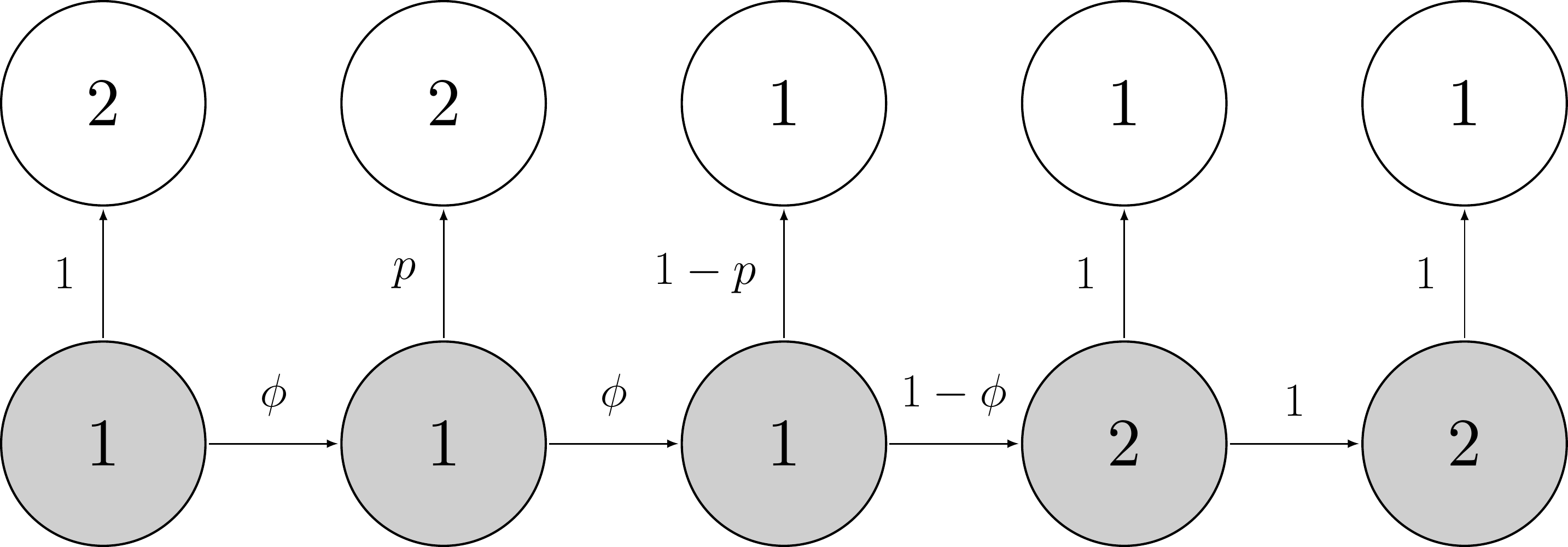
If we denote first the time of first detection, then our model so far is written as follows:

\[\begin{align*} z_{\text{first}} &\sim \text{Categorical}(1, \delta) &\text{[likelihood]}\\ z_t | z_{t-1} &\sim \text{Categorical}(1, \gamma_{z_{t-1},z_{t}}) &\text{[likelihood, t>first]}\\ y_t | z_{t} &\sim \text{Categorical}(1, \omega_{z_{t}}) &\text{[likelihood, t>first]}\\ \phi &\sim \text{Beta}(1, 1) &\text{[prior for }\phi \text{]} \\ p &\sim \text{Beta}(1, 1) &\text{[prior for }p \text{]} \\ \end{align*}\]

It has an observation layer for the \(y\)’s, conditional on the \(z\)’s. We also consider uniform priors for the detection and survival probabilities. How to implement this model in NIMBLE?

We start with priors for survival and detection probabilities:

hmm.survival <- nimbleCode({
  phi ~ dunif(0, 1) # prior survival
  p ~ dunif(0, 1) # prior detection
...

Then we define initial states, transition and observation matrices:

...
  # parameters
  delta[1] <- 1          # Pr(alive t = first) = 1
  delta[2] <- 0          # Pr(dead t = first) = 0
  gamma[1,1] <- phi      # Pr(alive t -> alive t+1)
  gamma[1,2] <- 1 - phi  # Pr(alive t -> dead t+1)
  gamma[2,1] <- 0        # Pr(dead t -> alive t+1)
  gamma[2,2] <- 1        # Pr(dead t -> dead t+1)
  omega[1,1] <- 1 - p    # Pr(alive t -> non-detected t)
  omega[1,2] <- p        # Pr(alive t -> detected t)
  omega[2,1] <- 1        # Pr(dead t -> non-detected t)
  omega[2,2] <- 0        # Pr(dead t -> detected t)
...

Then the likelihood:

...
    # likelihood
    for (i in 1:N){
    z[i,1] ~ dcat(delta[1:2])
    for (j in 2:T){
      z[i,j] ~ dcat(gamma[z[i,j-1], 1:2])
      y[i,j] ~ dcat(omega[z[i,j], 1:2])
    }
  }
})

The loop over time for each individual for (j in 2:T){} starts after the first time individuals are detected (this is time 2 for all of them here), because we work conditional on the first detection.

Overall, the code looks like:

hmm.survival <- nimbleCode({
  phi ~ dunif(0, 1) # prior survival
  p ~ dunif(0, 1) # prior detection
  # likelihood
  delta[1] <- 1          # Pr(alive t = first) = 1
  delta[2] <- 0          # Pr(dead t = first) = 0
  gamma[1,1] <- phi      # Pr(alive t -> alive t+1)
  gamma[1,2] <- 1 - phi  # Pr(alive t -> dead t+1)
  gamma[2,1] <- 0        # Pr(dead t -> alive t+1)
  gamma[2,2] <- 1        # Pr(dead t -> dead t+1)
  omega[1,1] <- 1 - p    # Pr(alive t -> non-detected t)
  omega[1,2] <- p        # Pr(alive t -> detected t)
  omega[2,1] <- 1        # Pr(dead t -> non-detected t)
  omega[2,2] <- 0        # Pr(dead t -> detected t)
  for (i in 1:N){
    z[i,1] ~ dcat(delta[1:2])
    for (j in 2:T){
      z[i,j] ~ dcat(gamma[z[i,j-1], 1:2])
      y[i,j] ~ dcat(omega[z[i,j], 1:2])
    }
  }
})

Now we specify the constants:

my.constants <- list(N = nrow(y), T = 5)
my.constants
## $N
## [1] 57
## 
## $T
## [1] 5

The data are made of 0’s for non-detections and 1’s for detections. To use the categorical distribution, we need to code 1’s and 2’s. We simply add 1 to get the correct format, that is \(y = 1\) for non-detection and \(y = 2\) for detection:

my.data <- list(y = y + 1)

Now let’s write a function for the initial values:

zinits <- y + 1 # non-detection -> alive
zinits[zinits == 2] <- 1 # dead -> alive
initial.values <- function() list(phi = runif(1,0,1),
                                  p = runif(1,0,1),
                                  z = zinits)

As initial values for the latent states, we assumed that whenever an individual was non-detected, it was alive, with with zinits <- y + 1, and we make sure dead individuals are alive with zinits[zinits == 2] <- 1.

We specify the parameters we’d like to monitor:

parameters.to.save <- c("phi", "p")
parameters.to.save
## [1] "phi" "p"

We provide MCMC details:

n.iter <- 5000
n.burnin <- 1000
n.chains <- 2

At last, we’re ready to run NIMBLE:

start_time <- Sys.time()
mcmc.output <- nimbleMCMC(code = hmm.survival,
                          constants = my.constants,
                          data = my.data,
                          inits = initial.values,
                          monitors = parameters.to.save,
                          niter = n.iter,
                          nburnin = n.burnin,
                          nchains = n.chains)
end_time <- Sys.time()
end_time - start_time

## Time difference of 12.27 secs

We can have a look to numerical summaries:

MCMCsummary(mcmc.output, round = 2)
##     mean   sd 2.5%  50% 97.5% Rhat n.eff
## p   0.61 0.06 0.50 0.61  0.72    1   740
## phi 0.75 0.04 0.67 0.75  0.83    1   805

The estimates for survival and detection are close to true survival \(\phi = 0.8\) and detection \(p = 0.6\) with which we simulated the data. The code I used is:

set.seed(2022) # for reproducibility
nocc <- 5 # nb of winters or sampling occasions
nind <- 57 # nb of animals
p <- 0.6 # detection prob
phi <- 0.8 # survival prob
# Vector of initial states probabilities
delta <- c(1,0) # all individuals are alive in first winter
# Transition matrix
Gamma <- matrix(NA, 2, 2)
Gamma[1,1] <- phi      # Pr(alive t -> alive t+1)
Gamma[1,2] <- 1 - phi  # Pr(alive t -> dead t+1)
Gamma[2,1] <- 0        # Pr(dead t -> alive t+1)
Gamma[2,2] <- 1        # Pr(dead t -> dead t+1)
# Observation matrix 
Omega <- matrix(NA, 2, 2)
Omega[1,1] <- 1 - p      # Pr(alive t -> non-detected t)
Omega[1,2] <- p          # Pr(alive t -> detected t)
Omega[2,1] <- 1          # Pr(dead t -> non-detected t)
Omega[2,2] <- 0          # Pr(dead t -> detected t)
# Matrix of states
z <- matrix(NA, nrow = nind, ncol = nocc)
y <- z
y[,1] <- 2 # all individuals are detected in first winter, as we condition on first detection
for (i in 1:nind){
  z[i,1] <- rcat(n = 1, prob = delta) # 1 for sure
  for (t in 2:nocc){
    # state at t given state at t-1
    z[i,t] <- rcat(n = 1, prob = Gamma[z[i,t-1],1:2]) 
    # observation at t given state at t
    y[i,t] <- rcat(n = 1, prob = Omega[z[i,t],1:2]) 
  }
}
y
y <- y - 1 # non-detection = 0, detection = 1

3.8 Marginalization

In some situations, you will not be interested in inferring the hidden states \(z_{i,t}\), so why bother estimating them? The good news is that you can get rid of the states, so that the marginal likelihood is a function of survival and detection probabilities \(\phi\) and \(p\) only.

3.8.1 Brute-force approach

Using the formula of total probability, you get the marginal likelihood by summing over all possible states in the complete likelihood:

\[\begin{align*} \Pr(\mathbf{y}_i) &= \Pr(y_{i,1}, y_{i,2}, \ldots, y_{i,T})\\ &= \sum_{\mathbf{z}_i} \Pr(\mathbf{y}_i, \mathbf{z}_i)\\ &= \sum_{z_{i,1}} \cdots \sum_{z_{i,T}} \Pr(y_{i,1}, y_{i,2}, \ldots, y_{i,T}, z_{i,1}, z_{i,2}, \ldots, z_{i,T})\\ \end{align*}\]

Going through the same steps as for deriving the complete likelihood, we obtain the marginal likelihood:

\[\begin{align*} \Pr(\mathbf{y}_i) &= \sum_{z_{i,1}} \cdots \sum_{z_{i,T}} \left(\prod_{t=1}^T{\omega_{z_{i,t}, y_{i,t}}}\right) \left(\Pr(z_{i,1}) \prod_{t=2}^T{\gamma_{z_{i,t-1},z_{i,t}}}\right)\\ \end{align*}\]

Let’s go through an example. Let’s imagine we have \(T = 3\) winters, and we’d like to write the likelihood for an individual having the encounter history detected, detected then non-detected. Remember that non-detected is coded 1 and detected is coded 2, while alive is coded 1 and dead is coded 2. We need to calculate \(\Pr(y_1 = 2, y_2 = 2, y_3 = 1)\) which, according to the formula above, is given by:

\[\begin{align*} \begin{split} \Pr(y_1 = 2, y_2 = 2, y_3 = 1) &= \sum_{i=1}^{2} \sum_{j=1}^{2} \sum_{k=1}^{2} \Pr(y_1 = 2 | z_1 = i) \Pr(y_2 = 2 | z_2 = j) \Pr(y_3 = 1 | z_3 = k) \\ & \qquad \Pr(z_1=i) \Pr(z_2 = j | z_1 = i) \Pr(z_3 = k | z_2 = j)\\ \end{split} \end{align*}\]

Expliciting all the sums in \(\Pr(y_1 = 2, y_2 = 2, y_3 = 1)\), we get the long and ugly expression:

\[\begin{align*} \begin{split} \Pr(y_1 = 2, y_2 = 2, y_3 = 1) &= \\ & \Pr(y_1 = 2 | z_1 = 1) \Pr(y_2 = 2 | z_2 = 1) \Pr(y_3 = 1 | z_3 = 1) \times \\ & \qquad \Pr(z_1 = 1) \Pr(z_2 = 1 | z_1 = 1) \Pr(z_3 = 1 | z_2 = 1) +\\ & \Pr(y_1 = 2 | z_1 = 2) \Pr(y_2 = 2 | z_2 = 1) \Pr(y_3 = 1 | z_3 = 1) \times\\ & \qquad \Pr(z_1 = 2) \Pr(z_2 = 1 | z_1 = 2) \Pr(z_3 = 1 | z_2 = 1) +\\ & \Pr(y_1 = 2 | z_1 = 1) \Pr(y_2 = 2 | z_2 = 2) \Pr(y_3 = 1 | z_3 = 1) \times\\ & \qquad \Pr(z_1 = 1) \Pr(z_2 = 2 | z_1 = 1) \Pr(z_3 = 1 | z_2 = 2) +\\ & \Pr(y_1 = 2 | z_1 = 2) \Pr(y_2 = 2 | z_2 = 2) \Pr(y_3 = 1 | z_3 = 1) \times\\ & \qquad \Pr(z_1 = 2) \Pr(z_2 = 2 | z_1 = 2) \Pr(z_3 = 1 | z_2 = 2) +\\ & \Pr(y_1 = 2 | z_1 = 1) \Pr(y_2 = 2 | z_2 = 1) \Pr(y_3 = 1 | z_3 = 2) \times\\ & \qquad \Pr(z_1 = 1) \Pr(z_2 = 1 | z_1 = 1) \Pr(z_3 = 2 | z_2 = 1) +\\ & \Pr(y_1 = 2 | z_1 = 2) \Pr(y_2 = 2 | z_2 = 1) \Pr(y_3 = 1 | z_3 = 2) \times\\ & \qquad \Pr(z_1 = 2) \Pr(z_2 = 1 | z_1 = 2) \Pr(z_3 = 2 | z_2 = 1) +\\ & \Pr(y_1 = 2 | z_1 = 1) \Pr(y_2 = 2 | z_2 = 2) \Pr(y_3 = 1 | z_3 = 2) \times\\ & \qquad \Pr(z_1 = 1) \Pr(z_2 = 2 | z_1 = 1) \Pr(z_3 = 2 | z_2 = 2) +\\ & \Pr(y_1 = 2 | z_1 = 2) \Pr(y_2 = 2 | z_2 = 2) \Pr(y_3 = 1 | z_3 = 2) \times\\ & \qquad \Pr(z_1 = 2) \Pr(z_2 = 2 | z_1 = 2) \Pr(z_3 = 2 | z_2 = 2)\\ \end{split} \end{align*}\]

You can simplify this expression by noticing that i) all individuals are alive for sure when marked and released in first winter, or \(\Pr(z_1=2) = 0\) and ii) dead individuals are non-detected for sure, or \(\Pr(y_t = 2|z_t = 2) = 0\), which lead to:

\[\begin{align*} \begin{split} \Pr(y_1 = 2, y_2 = 2, y_3 = 1) &= \\ & \Pr(y_1 = 2 | z_1 = 1) \Pr(y_2 = 2 | z_2 = 1) \Pr(y_3 = 1 | z_3 = 1) \times \\ & \qquad \Pr(z_1 = 1) \Pr(z_2 = 1 | z_1 = 1) \Pr(z_3 = 1 | z_2 = 1) +\\ & \Pr(y_1 = 2 | z_1 = 1) \Pr(y_2 = 2 | z_2 = 1) \Pr(y_3 = 1 | z_3 = 2) \times\\ & \qquad \Pr(z_1 = 1) \Pr(z_2 = 1 | z_1 = 1) \Pr(z_3 = 2 | z_2 = 1)\\ \end{split} \end{align*}\]

Because all individuals are captured in first winter, or \(\Pr(y_1 = 2 | z_1 = 1) = 1\), we get:

\[\begin{align*} \Pr(y_1 = 2, y_2 = 2, y_3 = 1) = 1 (1-p) \times 1 \phi \phi + 1 p 1 \times 1 \phi (1-\phi) \end{align*}\]

You end up with \(\Pr(y_1 = 2, y_2 = 2, y_3 = 1) = \phi p (1 - p\phi)\).

The latent states are no longer involved in the likelihood for this individual. However, even on a rather simple example, the marginal likelihood is quite complex to evaluate because it involves many operations. If \(T\) is the length of our encounter histories and \(N\) is the number of hidden states (two for alive and dead, but we will deal with more states in some chapters to come), then we need to calculate the sum of \(N^T\) terms (the sums in the formula above), each of which has two products of \(T\) factors (the products in the formula above), hence \(2TN^T\) calculations in total. You can check that in the simple example above, we have \(T^N = 2^3 = 8\) terms that are summed, each of which is a product of \(2T = 2 \times 3 = 6\) terms. This means that the number of operations increases exponentially as the number of states increases. In most cases, this complexity precludes using this method to get rid of the states. Fortunately, we have another algorithm in the HMM toolbox that is useful to calculate the marginal likelihood efficiently.

3.8.2 Forward algorithm

In the brute-force approach, some products are computed several times to calculate the marginal likelihood. What if we could store these products and use them later while computing the probability of the observation sequence? This is precisely what the forward algorithm does.

We introduce \(\alpha_t(j)\) the probability for the latent state \(z\) of being in state \(j\) at \(t\) after seeing the first \(j\) observations \(y_1, \ldots, y_t\), that is \(\alpha_t(j) = \Pr(y_1, \ldots, y_t, z_t = j)\).

Using the law of total probability, we can write the marginal likelihood as a function of \(\alpha_T(j)\), namely we have \(\Pr(\mathbf{y}) = \displaystyle{\sum_{j=1}^N\Pr(y_1, \ldots, y_t, z_t = j)} = \displaystyle{\sum_{j=1}^N\alpha_T(j)}\).

How to calculate the the \(\alpha_T(j)\)s? This is where the magic of the forward algorithm happens. We use a recurrence relationship that saves us many computations.

The recurrence states that:

\[\begin{align*} \alpha_t(j) &= \sum_{i=1}^N \alpha_{t-1}(i) \gamma_{i,j} \omega_{j,y_t} \end{align*}\]

How to obtain this recurrence? First, using the law of total probability with \(z_{t-1}\), we have that: \[\begin{align*} \alpha_t(j) &= \sum_{i=1}^N \Pr(y_1, \ldots, y_t, z_{t-1} = i, z_t = j)\\ \end{align*}\]

Second, using conditional probabilities, we get: \[\begin{align*} \alpha_t(j) &= \sum_{i=1}^N \Pr(y_t | z_{t-1} = i, z_t = j, y_1, \ldots, y_t) \Pr(z_{t-1} = i, z_t = j, y_1, \ldots, y_t) \end{align*}\]

Third, using conditional probabilities again, on the second term of the product, we get: \[\begin{align*} \alpha_t(j) &= \sum_{i=1}^N \Pr(y_t | z_{t-1} = i, z_t = j, y_1, \ldots, y_t) \times \\ & \Pr(z_t = j | z_{t-1} = i, y_1, \ldots, y_t) \Pr(z_{t-1} = i, y_1, \ldots, y_t) \end{align*}\]

which, using conditional independence, simplifies into:

\[\begin{align*} \alpha_t(j) &= \sum_{i=1}^N \Pr(y_t | z_t = j) \Pr(z_t = j | z_{t-1} = i) \Pr(z_{t-1} = i, y_1, \ldots, y_t) \end{align*}\]

Recognizing that \(\Pr(y_{t}|z_{t}=j)=\omega_{j,y_t}\), \(\Pr(z_{t} = j | z_{t-1} = i) = \gamma_{i,j}\) and \(\Pr(z_{t-1} = i, y_1, \ldots, y_t) = \alpha_{t-1}(i)\), we obtain the recurrence.

In practice, the forward algorithm works as follows. First you initialize the procedure by calculating for the states \(j=1,\ldots,N\) the quantities \(\alpha_1(j) = Pr(z_1 = j) \omega_{j,y_1}\). Then you compute for the states \(j=1,\ldots,N\) the relationship \(\alpha_t(j) = \displaystyle{\sum_{i=1}^N \alpha_{t-1}(i) \gamma_{i,j} \omega_{j,y_t}}\) for \(t = 2, \ldots, T\). Finally, you compute the marginal likelihood as \(\Pr(\mathbf{y}) = \displaystyle{\sum_{j=1}^N\alpha_T(j)}\). At each time \(t\), we need to calculate \(N\) values of \(\alpha_t(j)\), and each \(\alpha_t(j)\) is a sum of \(N\) products of \(\alpha_{t-1}\), \(\gamma_{i,j}\) and \(\omega_{j,y_t}\), hence \(TN^2\) computations in total, which is much less than the \(2TN^T\) calculations in the brute-force approach.

Going back to our example, we wish to calculate \(\Pr(y_1 = 2, y_2 = 2, y_3 = 1)\). First we initialize and compute \(\alpha_1(1)\) and \(\alpha_1(2)\). We have:

\[\begin{align*} \alpha_1(1) = \Pr(z_1=1) \omega_{1,y_1=2} = 1 \end{align*}\]

because all animals are alive and captured in first winter. We also have:

\[\begin{align*} \alpha_1(2) = \Pr(z_1=2) \omega_{2,y_1=2} = 0 \end{align*}\]

Then we compute \(\alpha_2(1)\) and \(\alpha_2(2)\). We have:

\[\begin{align*} \alpha_2(1) &= \sum_{i=1}^2 \alpha_1(i) \gamma_{i,1} \omega_{1,y_2=2}\\ &= \gamma_{1,1} \omega_{1,y_2=2}\\ &= \phi p \end{align*}\]

because \(\alpha_1(2) = 0\). Also, we have:

\[\begin{align*} \alpha_2(2) &= \sum_{i=1}^2 \alpha_1(i) \gamma_{i,2} \omega_{2,y_2=2}\\ &= \gamma_{1,2} \omega_{2,y_2=2}\\ &= (1-\phi) 0 \end{align*}\]

Finally we compute \(\alpha_3(1)\) and \(\alpha_3(2)\). We have:

\[\begin{align*} \alpha_3(1) &= \sum_{i=1}^2 \alpha_2(i) \gamma_{i,1} \omega_{1,y_3=1}\\ &= \alpha_2(1) \gamma_{1,1} \omega_{1,y_3=1}\\ &= \phi p \phi (1-p) \end{align*}\]

and:

\[\begin{align*} \alpha_3(2) &= \sum_{i=1}^2 \alpha_2(i) \gamma_{i,2} \omega_{2,y_3=1}\\ &= \alpha_2(1) \gamma_{1,2} \omega_{2,y_3=1}\\ &= \phi p (1-\phi) 1 \end{align*}\]

Eventually, we compute \(\Pr(y_1=2,y_2=2,y_3=1)\):

\[\begin{align*} \Pr(y_1=2,y_2=2,y_3=1) &= \alpha_3(1) + \alpha_3(2)\\ &= \phi p (\phi) (1-p) + \phi p (1-\phi)\\ &= \phi p (1-\phi p) \end{align*}\]

You can check that we did in total \(3 \times 2^2 = 12\) operations.

3.8.3 NIMBLE implementation

3.8.3.1 Do it yourself

In NIMBLE, we use functions to implement the forward algorithm. The only differences with the theory above is that i) we work on the log scale for numerical stability and ii) we use a matrix formulation of the recurrence.

First we write the density function:

dHMM <- nimbleFunction(
  run = function(x = double(1), 
                 probInit = double(1), # vector of initial states
                 probObs = double(2), #observation matrix
                 probTrans = double(2), # transition matrix
                 len = double(0, default = 0), # number of sampling occasions
                 log = integer(0, default = 0)) {
    alpha <- probInit[1:2] # * probObs[1:2,x[1]] == 1 due to conditioning on first detection
    for (t in 2:len) {
      alpha[1:2] <- (alpha[1:2] %*% probTrans[1:2,1:2]) * probObs[1:2,x[t]]
    }
    logL <- log(sum(alpha[1:2]))
    returnType(double(0))
    if (log) return(logL)
    return(exp(logL))
  }
)

In passing, this is the function you would maximize in a frequentist approach (see Section 2.5). Then we write a function to simulate values from a HMM:

rHMM <- nimbleFunction(
  run = function(n = integer(),
                 probInit = double(1),
                 probObs = double(2),
                 probTrans = double(2),
                 len = double(0, default = 0)) {
    returnType(double(1))
    z <- numeric(len)
    z[1] <- rcat(n = 1, prob = probInit[1:2]) # all individuals alive at t = 0
    y <- z
    y[1] <- 2 # all individuals are detected at t = 0
    for (t in 2:len){
      # state at t given state at t-1
      z[t] <- rcat(n = 1, prob = probTrans[z[t-1],1:2]) 
      # observation at t given state at t
      y[t] <- rcat(n = 1, prob = probObs[z[t],1:2]) 
    }
    return(y)
  })

We assign these functions to the global R environment:

assign('dHMM', dHMM, .GlobalEnv)
assign('rHMM', rHMM, .GlobalEnv)

Now we resume our workflow:

# code
hmm.survival <- nimbleCode({
  phi ~ dunif(0, 1) # prior survival
  p ~ dunif(0, 1) # prior detection
  # likelihood
  delta[1] <- 1          # Pr(alive t = 1) = 1
  delta[2] <- 0          # Pr(dead t = 1) = 0
  gamma[1,1] <- phi      # Pr(alive t -> alive t+1)
  gamma[1,2] <- 1 - phi  # Pr(alive t -> dead t+1)
  gamma[2,1] <- 0        # Pr(dead t -> alive t+1)
  gamma[2,2] <- 1        # Pr(dead t -> dead t+1)
  omega[1,1] <- 1 - p    # Pr(alive t -> non-detected t)
  omega[1,2] <- p        # Pr(alive t -> detected t)
  omega[2,1] <- 1        # Pr(dead t -> non-detected t)
  omega[2,2] <- 0        # Pr(dead t -> detected t)
  for (i in 1:N){
    y[i,1:T] ~ dHMM(probInit = delta[1:2], 
                    probObs = omega[1:2,1:2], # observation matrix
                    probTrans = gamma[1:2,1:2], # transition matrix
                    len = T) # nb of sampling occasions
  }
})
# constants
my.constants <- list(N = nrow(y), T = 5)
# data
my.data <- list(y = y + 1)
# initial values - no need to specify values for z anymore
initial.values <- function() list(phi = runif(1,0,1),
                                  p = runif(1,0,1))
# parameters to save
parameters.to.save <- c("phi", "p")
# MCMC details
n.iter <- 5000
n.burnin <- 1000
n.chains <- 2

And run NIMBLE:

start_time <- Sys.time()
mcmc.output <- nimbleMCMC(code = hmm.survival,
                          constants = my.constants,
                          data = my.data,
                          inits = initial.values,
                          monitors = parameters.to.save,
                          niter = n.iter,
                          nburnin = n.burnin,
                          nchains = n.chains)
## |-------------|-------------|-------------|-------------|
## |-------------------------------------------------------|
## |-------------|-------------|-------------|-------------|
## |-------------------------------------------------------|
end_time <- Sys.time()
end_time - start_time
## Time difference of 11.91 secs

The numerical summaries are similar to those we obtained with the complete likelihood, and effective samples sizes are larger denoting better mixing:

MCMCsummary(mcmc.output, round = 2)
##     mean   sd 2.5%  50% 97.5% Rhat n.eff
## p   0.61 0.06 0.49 0.61  0.72    1  1211
## phi 0.76 0.04 0.67 0.76  0.84    1  1483

3.8.3.2 Do it with nimbleEcology

Writing NIMBLE functions is not easy. Fortunately, the NIMBLE folks got you covered. They developed the package nimbleEcology that implements some of the most popular ecological models with latent states.

We will use the function dHMMo which provides the distribution of a hidden Markov model with time-independent transition matrix and time-dependent observation matrix. Why time-dependent observation matrix? Because we need to tell NIMBLE that detection at first encounter is 1.

We load the package:

library(nimbleEcology)

The NIMBLE code is:

hmm.survival <- nimbleCode({
  phi ~ dunif(0, 1) # prior survival
  p ~ dunif(0, 1) # prior detection
  # likelihood
  delta[1] <- 1          # Pr(alive t = 1) = 1
  delta[2] <- 0          # Pr(dead t = 1) = 0
  gamma[1,1] <- phi      # Pr(alive t -> alive t+1)
  gamma[1,2] <- 1 - phi  # Pr(alive t -> dead t+1)
  gamma[2,1] <- 0        # Pr(dead t -> alive t+1)
  gamma[2,2] <- 1        # Pr(dead t -> dead t+1)
  omega[1,1,1] <- 0        # Pr(alive first -> non-detected first)
  omega[1,2,1] <- 1        # Pr(alive first -> detected first)
  omega[2,1,1] <- 1        # Pr(dead first -> non-detected first)
  omega[2,2,1] <- 0        # Pr(dead first -> detected first)
  for (t in 2:5){
    omega[1,1,t] <- 1 - p    # Pr(alive t -> non-detected t)
    omega[1,2,t] <- p        # Pr(alive t -> detected t)
    omega[2,1,t] <- 1        # Pr(dead t -> non-detected t)
    omega[2,2,t] <- 0        # Pr(dead t -> detected t)
  }
  for (i in 1:N){
    y[i,1:5] ~ dHMMo(init = delta[1:2], # vector of initial state probabilities
                     probObs = omega[1:2,1:2,1:5], # observation matrix
                     probTrans = gamma[1:2,1:2], # transition matrix
                     len = 5, # nb of sampling occasions
                     checkRowSums = 0) # skip validity checks
  }
})

You may see that we no longer have the states in the code as we use the marginalized likelihood. The dHMMo takes several arguments, including init the vector of initial state probabilities, probObs the observation matrix, probTrans the transition matrix and len the number of sampling occasions.

Next steps are similar to the workflow we used before. The only difference is that we do not need to specify initial values for the latent states:

# constants
my.constants <- list(N = nrow(y))
# data
my.data <- list(y = y + 1)
# initial values - no need to specify values for z anymore
initial.values <- function() list(phi = runif(1,0,1),
                                  p = runif(1,0,1))
# parameters to save
parameters.to.save <- c("phi", "p")
# MCMC details
n.iter <- 5000
n.burnin <- 1000
n.chains <- 2

Now we run NIMBLE:

start_time <- Sys.time()
mcmc.output <- nimbleMCMC(code = hmm.survival,
                          constants = my.constants,
                          data = my.data,
                          inits = initial.values,
                          monitors = parameters.to.save,
                          niter = n.iter,
                          nburnin = n.burnin,
                          nchains = n.chains)
## |-------------|-------------|-------------|-------------|
## |-------------------------------------------------------|
## |-------------|-------------|-------------|-------------|
## |-------------------------------------------------------|
end_time <- Sys.time()
end_time - start_time
## Time difference of 12.35 secs

Now we display the numerical summaries of the posterior distributions:

MCMCsummary(mcmc.output, round = 2)
##     mean   sd 2.5%  50% 97.5% Rhat n.eff
## p   0.61 0.06 0.49 0.61  0.72    1  1453
## phi 0.76 0.04 0.67 0.76  0.84    1  1359

The results are similar what we obtained previously with our home-made marginalized likelihood (Section 3.8.3.1), or with the full likelihood (3.7).

3.9 Pooled encounter histories

We can go one step further to make convergence even faster. As mentionned earlier in Section 3.6.4, the likelihood of an HMM fitted to capture-recapture data often involves individuals that share the same encounter histories. Instead of repeating the same calculations several times, the likelihood contribution that is shared by say \(x\) individuals is raised to the power \(x\) in the likelihood of the whole dataset, hence making the same operations only once. This idea is used in routine in capture-recapture software. For Bayesian software however, it is only recently that the trick was tested in NIMBLE by Turek, de Valpine, and Paciorek (2016).

In this section, we amend the NIMBLE functions we wrote for marginalizing latent states in Section 3.8 to express the likelihood using pooled encounter histories. We use a vector size that contains the number of individuals with the same encounter history.

The density function is the function dHMM to which we add a size argument, and raise the individual likelihood to the power size, or multiply by size as we work on the log scale log(sum(alpha[1:2])) * size:

dHMMpooled <- nimbleFunction(
  run = function(x = double(1), 
                 probInit = double(1),
                 probObs = double(2),
                 probTrans = double(2),
                 len = double(0),
                 size = double(0),
                 log = integer(0, default = 0)) {
    alpha <- probInit[1:2]
    for (t in 2:len) {
      alpha[1:2] <- (alpha[1:2] %*% probTrans[1:2,1:2]) * probObs[1:2,x[t]]
    }
    logL <- log(sum(alpha[1:2])) * size
    returnType(double(0))
    if (log) return(logL)
    return(exp(logL))
  }
)

The rHMM function is renamed rHMMpooled for compatibility but remains unchanged:

rHMMpooled <- nimbleFunction(
  run = function(n = integer(),
                 probInit = double(1),
                 probObs = double(2),
                 probTrans = double(2),
                 len = double(0),
                 size = double(0)) {
    returnType(double(1))
    z <- numeric(len)
    z[1] <- rcat(n = 1, prob = probInit[1:2]) # all individuals alive at t = 0
    y <- z
    y[1] <- 2 # all individuals are detected at t = 0
    for (t in 2:len){
      # state at t given state at t-1
      z[t] <- rcat(n = 1, prob = probTrans[z[t-1],1:2]) 
      # observation at t given state at t
      y[t] <- rcat(n = 1, prob = probObs[z[t],1:2]) 
    }
    return(y)
  })

We assign these two function to the global R environment so that we can use them:

assign('dHMMpooled', dHMMpooled, .GlobalEnv)
assign('rHMMpooled', rHMMpooled, .GlobalEnv)

You can now plug your pooled HMM density function in your NIMBLE code:

hmm.survival <- nimbleCode({
  phi ~ dunif(0, 1) # prior survival
  p ~ dunif(0, 1) # prior detection
  # likelihood
  delta[1] <- 1          # Pr(alive t = 1) = 1
  delta[2] <- 0          # Pr(dead t = 1) = 0
  gamma[1,1] <- phi      # Pr(alive t -> alive t+1)
  gamma[1,2] <- 1 - phi  # Pr(alive t -> dead t+1)
  gamma[2,1] <- 0        # Pr(dead t -> alive t+1)
  gamma[2,2] <- 1        # Pr(dead t -> dead t+1)
  omega[1,1] <- 1 - p    # Pr(alive t -> non-detected t)
  omega[1,2] <- p        # Pr(alive t -> detected t)
  omega[2,1] <- 1        # Pr(dead t -> non-detected t)
  omega[2,2] <- 0        # Pr(dead t -> detected t)
  for (i in 1:N){
    y[i,1:T] ~ dHMMpooled(probInit = delta[1:2], 
                          probObs = omega[1:2,1:2], # observation matrix
                          probTrans = gamma[1:2,1:2], # transition matrix
                          len = T, # nb of sampling occasions
                          size = size[i]) # number of individuals with encounter history i
  }
})

Before running NIMBLE, we need to actually pool individuals with the same encounter history together:

y_pooled <- y %>% 
  as_tibble() %>% 
  group_by_all() %>% # group
  summarise(size = n()) %>% # count
  relocate(size) %>% # put size in front
  arrange(-size) %>% # sort along size
  as.matrix()
y_pooled
##       size winter 1 winter 2 winter 3 winter 4 winter 5
##  [1,]   21        1        0        0        0        0
##  [2,]    8        1        1        0        0        0
##  [3,]    8        1        1        1        1        0
##  [4,]    4        1        1        0        0        1
##  [5,]    4        1        1        1        0        0
##  [6,]    2        1        0        0        1        0
##  [7,]    2        1        0        1        1        0
##  [8,]    2        1        1        0        1        0
##  [9,]    1        1        0        1        0        0
## [10,]    1        1        0        1        0        1
## [11,]    1        1        0        1        1        1
## [12,]    1        1        1        0        1        1
## [13,]    1        1        1        1        0        1
## [14,]    1        1        1        1        1        1

For example, we have 21 individuals with encounter history (1, 0, 0, 0, 0).

Now you can resume the NIMBLE workflow:

my.constants <- list(N = nrow(y_pooled), T = 5, size = y_pooled[,'size'])
my.data <- list(y = y_pooled[,-1] + 1) # delete size from dataset
initial.values <- function() list(phi = runif(1,0,1),
                                  p = runif(1,0,1))
parameters.to.save <- c("phi", "p")
n.iter <- 5000
n.burnin <- 1000
n.chains <- 2
start_time <- Sys.time()
mcmc.output <- nimbleMCMC(code = hmm.survival,
                          constants = my.constants,
                          data = my.data,
                          inits = initial.values,
                          monitors = parameters.to.save,
                          niter = n.iter,
                          nburnin = n.burnin,
                          nchains = n.chains)
## |-------------|-------------|-------------|-------------|
## |-------------------------------------------------------|
## |-------------|-------------|-------------|-------------|
## |-------------------------------------------------------|
end_time <- Sys.time()
end_time - start_time
## Time difference of 11.09 secs
MCMCsummary(mcmc.output, round = 2)
##     mean   sd 2.5%  50% 97.5% Rhat n.eff
## p   0.61 0.06 0.49 0.61  0.72    1  1455
## phi 0.76 0.04 0.67 0.76  0.84    1  1524

The results are the same as those obtained previously. The gain in computation times will be bigger for more complex models as we will see in the next chapters.

The pooled likelihood is not yet implemented in nimbleEcology, but you can hack the code for the function dHMMo https://github.com/nimble-dev/nimbleEcology/blob/master/R/dHMM.R to implement it yourself by adding a size argument.

3.10 Decoding after marginalization

If you need to infer the latent states, and you cannot afford the computation times of the complete likelihood of Section 3.6.4, you can still use the marginal likelihood with the forward algorithm of Section 3.8.2. You will need an extra step to decode the latent states with the Viterbi algorithm. The Viterbi algorithm allows you to compute the sequence of states that is most likely to have generated the sequence of observations.

3.10.1 Theory

In our simulated dataset, animal #15 has the encounter history (2, 1, 1, 1, 1) which was generated from the sequence of states (1, 1, 2, 2, 2) with survival probability \(\phi = 0.8\) and detection probability \(p = 0.6\).

Imagine you do not know the truth. What is the chance that animal #15 was alive throughout the study when observing the encounter history detected in first winter, then missed in each subsequent winter? The chance of being alive in the first winter and detected when alive is 1. The chance of being alive in the second winter and non-detected is \(0.8 \times (1-0.6) = 0.32\). The same goes for third, fourth and fifth winters. In total, the probability of being alive throughout the study for an animal with encounter history (2, 1, 1, 1, 1) is \(1 \times 0.32 \times 0.32 \times 0.32 \times 0.32 = 0.01048576\).

Now what is the chance that animal #15 was alive, then dead for the rest of the study, when observing the encounter history (2, 1, 1, 1, 1)? And the chance of being alive in first and second winters, then dead after when observing the same encounter history? And so on. You need to enumerate all possible sequences of states and compute the probability for each of them, and choose the most probable sequence, that is with maximum probability. In our example, we would need to compute \(2^5 = 32\) of these probabilities, and \(N^T\) in general. Needless to say, these calculations quickly become cumbersome, if not impossible, as the number of states and/or the number of sampling occasions increases.

This is where the Viterbi algorithm comes in. The idea is to decompose this overall complex problem in a sequence of smallers problems that are easier to solve. If dynamic programming rings a bell, the Viterbi algorithm should look familiar to you. The Viterbi algorithm is based on the fact that the optimal path to each winter and each state can be deduced from the optimal path to the previous winter and each state.

For first winter, the probability of being alive and detected is 1, while the probability of being dead and detected is 0. Now what is the probability of being alive in the second winter and non-detected? If the animal was alive in the first winter, it remains alive and is missed with probability \(1 \times \phi (1-p) = 0.32\). If it was dead in the first winter, then this probability is 0. The maximum probability is 0.32 obviously so the most probable scenario to being alive in the second winter is being alive in the first winter. What about being dead in the second winter? If the animal was alive in first winter, then the probability is \(1 \times (1-\phi) \times 1 = 0.2\). If dead, then this probability is \(0 \times 0 \times (1-p) = 0\). The maximum probability is 0.2 obviously so the most probable scenario to being dead in the second winter is being alive in the first winter. Doing these calculations for third, fourth and fifth winters, we get the probabilities:

	winter 1	winter2	winter 3	winter 4	winter 5
state alive	1	0.32 = max(0, 0.32)	0.2304 = max(0, 0.2304)	0.110592 = max(0, 0.110592)	0.053084416 = max(0, 0.05308416
state dead	0	1 = max(1, 0.2)	1 = max(0.096, 1)	1 = max(0.04608, 1)	1 = max(0.0221184, 1)
observation	detected	missed	missed	missed	missed

Finally, to get (or decode) the optimal path, you work backwards and trace back the previous value that yielded the maximum probability. The most probable state in the last winter is dead (1 > 0.05308416), dead again in the fourth winter (1 > 0.110592), dead in the third winter (1 > 0.2304), alive in the second winter (1 > 0.48) and alive in the firt winter (1 > 0). According to the Viterbi algorithm, the sequence of states that most likelily generated the sequence of observations (2, 1, 1, 1, 1) is alive then dead, dead, dead and dead or (1 2 2 2 2). This differs slightly from the actual sequence of states (1, 1, 2, 2, 2) in that the state in second winter is decoded dead while animal #15 only dies in third winter.

In contrast to the brute force approach, calculations are not duplicated but stored and used again like in the forward algorithm. Briefly speaking, the Viterbi algorithm works like the forward algorithm where sums are replaced by calculating maximums.

In practice, the Viterbi algorithm works as illustrated in Figure 3.1. First you initialize the procedure by calculating at \(t=1\) for all states \(j=1,\ldots,N\) the values \(\nu_1(j) = Pr(z_1 = j) \omega_{j,y_1}\). Then you compute for all states \(j=1,\ldots,N\) the values \(\nu_t(j) = \displaystyle{\max_{i=1,\ldots,N} \nu_{t-1}(i) \gamma_{i,j} \omega_{j,y_t}}\) for \(t = 2, \ldots, T\). Here at each time \(t\) we determine the probability of the best path ending at each of the states \(j=1,\ldots,N\). Finally, you compute the probability of the best global path \(\displaystyle{\max_{j=1,\ldots,N}\nu_T(j)}\).

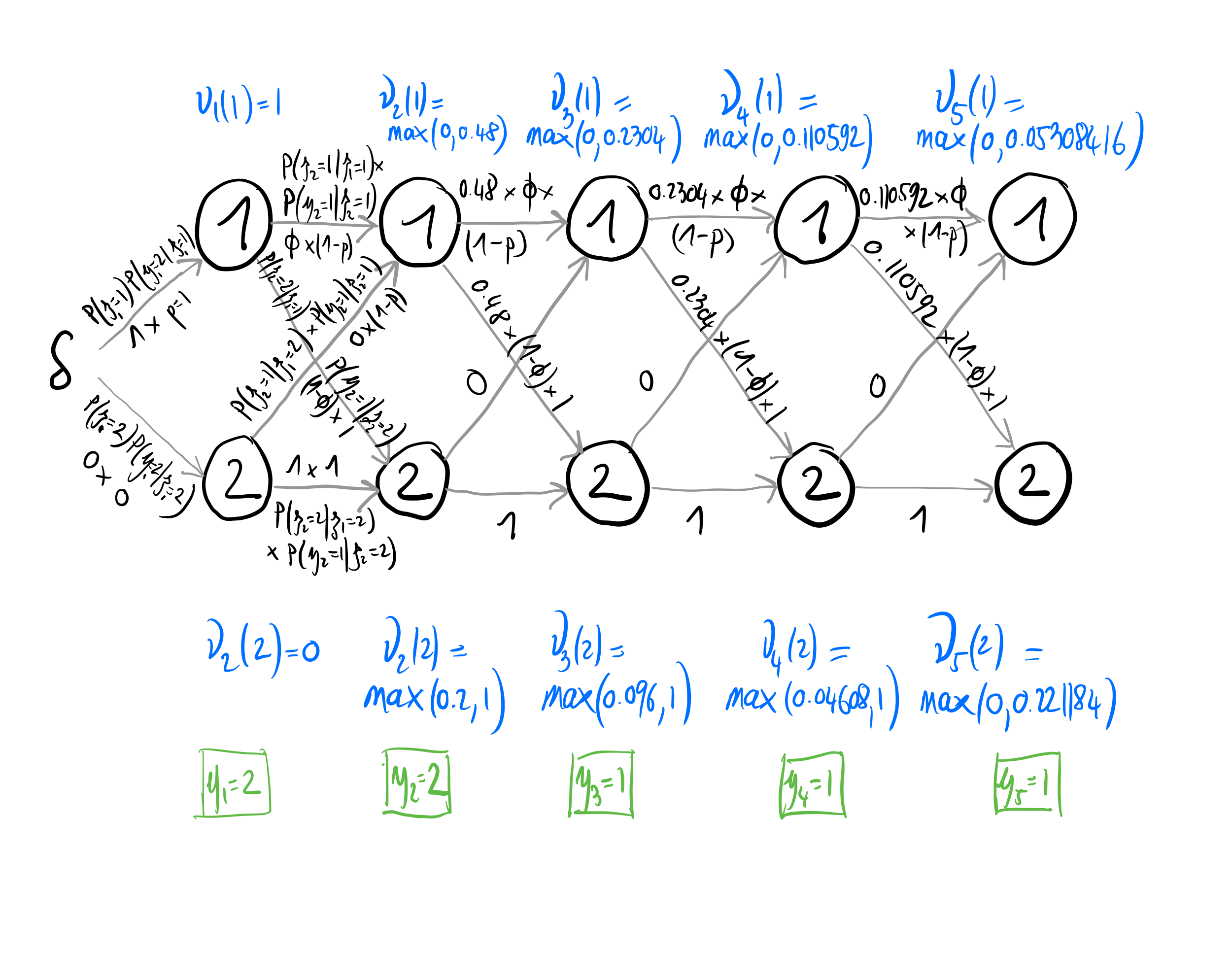
Figure 3.1: Graphical representation of the Viterbi algorithm with \(\phi = 0.8\) and \(p = 0.6\). States are alive \(z = 1\) or dead \(z = 2\) and observations are non-detected \(y = 1\) or detected \(y = 2\). To be done properly w/ tikz.

3.10.2 Implementation

Let’s write a R function to implement the Viterbi algorithm. As parameters, our function will take the transition and observation matrices, the vector of initial state probabilities and the observed sequence of detections and non-detections for which you aim to compute the sequence of states from which it was most likely generated:

# getViterbi() returns sequence of states that most likely generated sequence of observations
# adapted from https://github.com/vbehnam/viterbi
getViterbi <- function(Omega, Gamma, delta, y) {
# Omega: transition matrix
# Gamma: observation matrix
# delta: vector of initial state probabilities
# y: observed sequence of detections and non-detections
  
# get number of states and sampling occasions
N <- nrow(Gamma)
T <- length(y)
  
# nu is the corresponding likelihood
nu <- matrix(0, nrow = N, ncol = T)
# zz contains the most likely states up until this point
zz <- matrix(0, nrow = N, ncol = T)
firstObs <- y[1]
  
# fill in first columns of both matrices
#nu[,1] <- initial * emission[,firstObs]
#zz[,1] <- 0
nu[,1] <- c(1,0) # initial = (1, 0) * emission[,firstObs] = (1, 0)
zz[,1] <- 1 # alive at first occasion

for (i in 2:T) {
    for (j in 1:N) {
      obs <- y[i]
      # initialize to -1, then overwritten by for loop coz all possible values are >= 0
      nu[j,i] <- -1
      # loop to find max and argmax for k
      for (k in 1:N) {
        value <- nu[k,i-1] * Gamma[k,j] * Omega[j,obs]
        if (value > nu[j,i]) {
          # maximizing for k
          nu[j,i] <- value
          # argmaximizing for k
          zz[j,i] <- k
        }
      }
    }
  }
  # mlp = most likely path
  mlp <- numeric(T)
  # argmax for stateSeq[,T]
  am <- which.max(nu[,T])
  mlp[T] <- zz[am,T]
  
  # backtrace using backpointers
  for (i in T:2) {
    zm <- which.max(nu[,i])
    mlp[i-1] <- zz[zm,i]
  }
  return(mlp)
}

Note that instead of writing your own R function, you could use a built-in function from an existing R package to implement the Viterbi algorithm (for example, the viterbi() function from the HMM and depmixS4 packages), and call it from NIMBLE as we have seen in Section 2.4.2. The difficulty is that HMM for capture-recapture data have specific features that make standard functions not adapted and requires coding your own Viterbi function. In particular, we have to deal with detection at first encounter, which is not estimated but is always one because an individual has to be captured to be marked and released for the first time. Also, our transition and observation matrices are not always homogeneous and may depend on time.

Let’s test our getViterbi() function with our previous example. Remember animal #15 has the encounter history (2, 1, 1, 1, 1) which was generated from the sequence of states (1, 1, 2, 2, 2). Applying our function to that animal encounter history, we get:

delta # Vector of initial states probabilities
## [1] 1 0
Gamma # Transition matrix
##      [,1] [,2]
## [1,]  0.8  0.2
## [2,]  0.0  1.0
Omega # Observation matrix
##      [,1] [,2]
## [1,]  0.4  0.6
## [2,]  1.0  0.0
getViterbi(Omega = Omega, 
           Gamma = Gamma, 
           delta = delta, 
           y = y[15,] + 1)
## [1] 1 2 2 2 2

The Viterbi algorithm does pretty well at recovering the latent states, despite incorrectly decoding a death in the second winter while individual #15 only dies in the third winter. We obtained the same results by implementing the Viterbi algorithm by hand in Section 3.10.1.

Now that we have a function that implements the Viterbi algorithm, we can use it with our MCMC outputs. You have two options, either you apply Viterbi to each MCMC iteration then you compute the posterior median or mode path for each individual, or you compute the posterior mean or median of the transition and observation matrices then you apply Viterbi to each individual encounter history.

For both options, we will need the values from the posterior distributions of survival and detection probabilities:

phi <- c(mcmc.output$chain1[,'phi'], mcmc.output$chain2[,'phi'])
p <- c(mcmc.output$chain1[,'p'], mcmc.output$chain2[,'p'])

3.10.3 Compute first, average after

First option is to apply Viterbi to each MCMC sample, then to compute median of the MCMC Viterbi paths for each observed sequence:

niter <- length(p)
T <- 5
res <- matrix(NA, nrow = nrow(y), ncol = T)
for (i in 1:nrow(y)){
  res_mcmc <- matrix(NA, nrow = niter, ncol = T)
  for (j in 1:niter){
    # Initial states
    delta <- c(1, 0)
    # Transition matrix
    transition <- matrix(NA, 2, 2)
    transition[1,1] <- phi[j]      # Pr(alive t -> alive t+1)
    transition[1,2] <- 1 - phi[j]  # Pr(alive t -> dead t+1)
    transition[2,1] <- 0        # Pr(dead t -> alive t+1)
    transition[2,2] <- 1        # Pr(dead t -> dead t+1)
    # Observation matrix 
    emission <- matrix(NA, 2, 2)
    emission[1,1] <- 1 - p[j]      # Pr(alive t -> non-detected t)
    emission[1,2] <- p[j]          # Pr(alive t -> detected t)
    emission[2,1] <- 1          # Pr(dead t -> non-detected t)
    emission[2,2] <- 0          # Pr(dead t -> detected t)
    res_mcmc[j,1:T] <- getViterbi(emission, transition, delta, y[i,] + 1)
  }
  res[i, 1:length(y[1,])] <- apply(res_mcmc, 2, median)
}

You can compare the Viterbi decoding to the actual states \(z\):

Figure 3.2: Comparison of the actual sequences of states to the sequences of states decoded with Viterbi and the average first, compute after method.

Decoding is correct except that the alive actual state is often decoded as the dead state by the Viterbi algorithm. Note that here we compute the Viterbi paths after we run NIMBLE. You could turn the R function getViterbi() into a NIMBLE function and plug it in your model code to apply Viterbi. This would not make any difference except perhaps to increase MCMC computation times.

3.10.4 Average first, compute after

Second option is to compute the posterior mean of the observation and transition matrices, then to apply Viterbi:

# Initial states
delta <- c(1, 0)
# Transition matrix
transition <- matrix(NA, 2, 2)
transition[1,1] <- mean(phi)      # Pr(alive t -> alive t+1)
transition[1,2] <- 1 - mean(phi)  # Pr(alive t -> dead t+1)
transition[2,1] <- 0              # Pr(dead t -> alive t+1)
transition[2,2] <- 1              # Pr(dead t -> dead t+1)
# Observation matrix 
emission <- matrix(NA, 2, 2)
emission[1,1] <- 1 - mean(p)      # Pr(alive t -> non-detected t)
emission[1,2] <- mean(p)          # Pr(alive t -> detected t)
emission[2,1] <- 1                # Pr(dead t -> non-detected t)
emission[2,2] <- 0                # Pr(dead t -> detected t)
res <- matrix(NA, nrow = nrow(y), ncol = T)
for (i in 1:nrow(y)){
  res[i, 1:length(y[1,]) ] <- getViterbi(emission, transition, delta, y[i,] + 1)
}

Again, you can compare the result of the Viterbi decoding to the actual states we simulated and used to generate the observations:

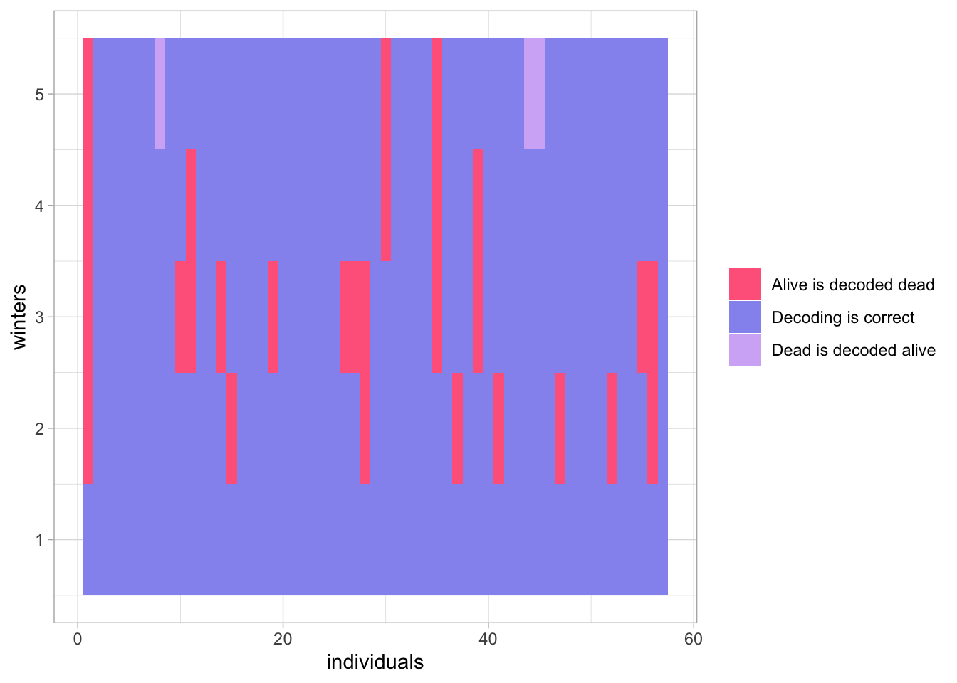
Figure 3.3: Comparison of the actual sequences of states to the sequences of states decoded with Viterbi and the compute first, average after approach.

The results are very similar to those we obtained in Section 3.10.3, and Figure 3.3 is indisguishable from Figure 3.2.

3.11 Summary

• A HMM is a model that consists of two parts: i) an unobserved sequence of discrete random variables - the states - satisfying the Markovian property (future states depends on current states only and not on past states) and ii) an observed sequence of discrete random variables - the observations - depending only on the current state.

• The Bayesian approach together with MCMC simulations allow estimating survival and detection probabilities as well as individual latent states alive or dead with the complete likelihood. If you can afford the computation times, then using the complete likelihood is the easiest path for model fitting.

• If you do not need to infer the latent states, you can use the marginal likelihood via the forward algorithm. By avoiding to sample the latent states, you usually get better mixing and faster convergence.

• If you do need to infer the latent states, and you cannot afford the computation times of the complete likelihood, then you can go for the marginal likelihood in conjunction with the Viterbi algorithm to decode the latent states.

• If the computational burden is still an issue, and you have individuals that share the same encounter history, you can use a pooled likelihood to speed up the marginal likelihood evaluation and MCMC convergence.

3.12 Suggested reading

• A landmark paper on HMM is Rabiner (1989).

• Check out Jurafsky and Martin (2023) for a nice introduction to HMM and Zucchini, MacDonald, and Langrock (2016) for an excellent book that covers theory and applications.

• The paper by McClintock et al. (2020) reviews the applications of HMM in ecology.

• The package nimbleEcology is developed by Goldstein et al. (2021) and Ponisio et al. (2020) for application to occupancy and N–mixture models.