6 Dealing with covariates

6.1 Introduction

Capture-recapture models often aim not just to estimate demographic parameters, but also to understand what drives their variation as we have seen in Chapter 4. Here, we will cover the selection of covariates from a potentially large set, using an extension of standard MCMC algorithms known as reversible jump MCMC (RJMCMC), and how to handle with uncertainty in key covariates, namely age or sex, when these are not perfectly known for all individuals.

6.2 Covariate selection with Reversible Jump MCMC

6.2.1 Motivation

In Section 4.6, we used WAIC to figure our which model, among several candidates, was best supported by the data. Each model there represented a different ecological hypothesis. Now when you are in a situation where you have several individual or temporal covariates that might explain variation in some demographic parameters, say survival as in Section 4.8, things can quickly become a bit more tedious. Let’s look at a real-world example with the white stork (Ciconia ciconia) population in Baden-Württemberg, Germany. From the 1960s to the 1990s, all Western European stork populations were in decline. One leading hypothesis was that these declines were driven by reduced food availability, itself caused by severe droughts in the storks’ wintering grounds in the Sahel region Grosbois et al. (2008).

To explore this idea, we’ll use rainfall measurements from 10 meteorological stations chosen to represent the storks’ wintering area: Diourbel, Gao, Kayes, Kita, Maradi, Mopti, Ouahigouya, Ségou, Tahoua, and Tombouctou. The data we have are the cumulative rainfall amounts (in mm) over June, July, August, and September – roughly the rainy season in the Sahel:

##      Diourbel  Gao Kayes  Kita Maradi Mopti Ouahigouya
## [1,]     6770 1900  7130 11350   6970  6580       6220
## [2,]     6420 2690  6180 13690   5880  6470       6260
## [3,]     6890 3530  6480 11820   6100  5230       6730
## [4,]     5700 2710  8440  9590   5210  5670       5670
## [5,]     6760 2090  6910  9850   6020  4200       5630
## [6,]     5432 2100  6300  8960   6890  3900       7180
##      Ségou Tahoua Tombouctou
## [1,]  8380   3920       1390
## [2,]  7530   3200       2210
## [3,]  6340   5170       1760
## [4,]  7490   4370       2580
## [5,]  5920   3120       2340
## [6,]  6461   3891       2020

Our question is: Which combination of these stations best explains variation in survival? If we tried to answer this by testing every possible model, we would have to consider every subset of the 10 stations and compare 1024 models (2^10 combinations). That’s far too many for a WAIC-based approach to be practical.

Instead of comparing all possible models one by one, we can use Reversible Jump MCMC (RJMCMC). RJMCMC is an extension of standard Bayesian inference in which the model itself is treated as an additional, discrete parameter. In this framework, the posterior distribution spans both the parameter space (e.g. regression coefficients) and the model space (e.g. which covariates are included). In simple terms, allows the algorithm to jump between models, switching covariates on or off as it goes. You can think of it as a hiker exploring different trails (models), stopping along each trail to take measurements (parameters) before deciding whether to move onto another path.

Using RJMCMC, we can estimate the posterior probability that each covariate influences survival, and obtain model-averaged regression coefficients and survival estimates that incorporate both parameter and model uncertainty.

We won’t dive into the mathematical details here but don’t worry, you can still follow the analysis without them. Check out Chapter 7 of King et al. (2009; see also Gimenez et al. 2009) if you’re interested in.

6.2.2 Model and NIMBLE implementation

For our example, we’ll work with data from 321 encounter histories of white storks ringed as chicks between 1956 and 1970. These data were kindly provided by Jean-Dominique Lebreton. We’ll fit a Cormack–Jolly–Seber (CJS) model with time-dependent survival and constant detection probability, as described in Section 4.5. We model the survival probability phi as a linear function of our covariates stored in x. To handle model selection inside the RJMCMC, we use a trick: for each covariate, we introduce an indicator variable ksi that can take the value 1 (covariate is included in the model) or 0 (covariate is excluded). We then combine the regression coefficients beta with these indicators into a single vector betaksi. This means that if ksi[j] = 0, the effect of covariate j is zero, effectively removing it from the model. Here’s how it works in the NIMBLE code:

for (t in 1:(T-1)){
  logit(phi[t]) <- intercept + inprod(betaksi[1:10], x[t, 1:10])
  gamma[1,1,t] <- phi[t]      # Pr(alive t -> alive t+1)
  gamma[1,2,t] <- 1 - phi[t]  # Pr(alive t -> dead t+1)
  gamma[2,1,t] <- 0           # Pr(dead t -> alive t+1)
  gamma[2,2,t] <- 1           # Pr(dead t -> dead t+1)
}

For the indicators and regression coefficients:

for (j in 1:10){
  betaksi[j] <- beta[j] * ksi[j]
  ksi[j] ~ dbern(psi) # indicator variable associated with betaj
}
psi ~ dbeta(1, 1) # prior on inclusion probability
for (j in 1:10){
  beta[j] ~ dnorm(0, sd = 1.5) # prior slopes
}
intercept ~ dnorm(0, sd = 1.5) # prior intercept

The prior on psi controls the overall tendency to include covariates in the model. Setting it to dbeta(1, 1) makes all inclusion probabilities equally likely, so the data drive the selection. The priors on beta and the intercept (not consider in the selection) are weakly informative.

As we saw in Section 2.6.1, NIMBLE allows you to change the default sampler. Here, we’re going to do something slightly different and use NIMBLE’s configureRJ() function to set up RJMCMC for variable selection. The function configureRJ() modifies an existing MCMC configuration so that RJMCMC is used to sample certain parameters, allowing covariates to be turned on or off during the run. It uses a univariate normal proposal distribution, and you can adjust the proposal mean and scale. The main arguments are:
- targetNodes: The parameters you want to apply variable selection to (e.g. beta);
- indicatorNodes: The indicator variables paired with the target nodes (e.g. ksi);
- control: A list for fine-tuning the proposal with mean the mean of the proposal distribution (default is 0), scale the standard deviation of the proposal (default is 1) and fixedValue the value a variable takes when excluded (default is 0).

Here’s how we apply it to our white stork example:

## Build the model and configure default MCMC
RJsurvival <- nimbleModel(code = hmm.phirjmcmcp, 
                          constants = my.constants,
                          data = my.data,
                          inits = initial.values())

Csurvival <- compileNimble(RJsurvival)

RJsurvivalConf <- configureMCMC(RJsurvival)
RJsurvivalConf$addMonitors('ksi')

# Switch to reversible jump sampling for the betas
configureRJ(conf = RJsurvivalConf,
            targetNodes = 'beta',
            indicatorNodes = 'ksi',
            control = list(mean = 0, scale = 2))

We then build, compile, and run the RJMCMC:

survivalMCMC <- buildMCMC(RJsurvivalConf)
CsurvivalMCMC <- compileNimble(survivalMCMC, project = RJsurvival)
samples <- runMCMC(mcmc = CsurvivalMCMC, 
                   niter = n.iter,
                   nburnin = n.burnin,
                   nchains = n.chains)

When we run this MCMC, configureRJ() takes care of proposing moves that either keep a covariate in the model or drop it out by setting its ksi value to 0. If a covariate is included (ksi = 1), the sampler updates its regression coefficient beta using the specified normal proposal distribution. If it’s excluded (ksi = 0), the coefficient is fixed at zero (our fixedValue). Over many iterations, the chain ‘jumps’ between different combinations of covariates, building up posterior probabilities for each one’s inclusion. This means we can later summarise which covariates are most likely to affect survival (via their inclusion probabilities), and model-averaged estimates of survival that incorporate the uncertainty about which covariates belong in the model. This is what we do in R in the next section.

6.2.3 Results and interpretation

The RJMCMC run gives us the posterior probabilities of different models where each model corresponds to a specific combination of covariates. To get these probabilities, we first combine the MCMC samples from our two chains:

# Gather two chains
out <- rbind(samples[[1]], samples[[2]])

Next, we look at the inclusion indicators ksi, which take value 1 if a covariate is in the model and 0 if not. The posterior mean of each ksi[j] is simply the estimated probability that covariate j is included:

# Number of covariates
K <- 10

# Extract only ksi columns, in order ksi[1], ..., ksi[10]
ksi <- out[, paste0("ksi[", 1:K, "]")]

# Posterior inclusion probabilities for each covariate
inclusion_prob <- colMeans(ksi)
inclusion_prob
##  ksi[1]  ksi[2]  ksi[3]  ksi[4]  ksi[5]  ksi[6]  ksi[7] 
## 0.02575 0.01720 0.01560 0.96120 0.04430 0.05350 0.02025 
##  ksi[8]  ksi[9] ksi[10] 
## 0.03360 0.02630 0.02965

The posterior inclusion probabilities tell us how likely each covariate is to appear in the ‘true’ model given the data and priors. Here, ksi[4] stands out, with an inclusion probability around 0.96. This corresponds to the the Kita station.

We can also identify the most probable models visited by the RJMCMC. Each MCMC draw corresponds to a model, which we encode as a binary string (e.g., “0101001001”):

# Encode each model draw as a string of 0s and 1s
model_id <- apply(ksi, 1, paste0, collapse = "")

# Empirical posterior model probabilities
post_model_prob <- sort(prop.table(table(model_id)), decreasing = TRUE)

# Show the top models
head(data.frame(model = names(post_model_prob), 
                prob = as.numeric(post_model_prob)), 10)
##         model    prob
## 1  0001000000 0.75470
## 2  0001010000 0.03965
## 3  0001100000 0.02910
## 4  0000000000 0.02310
## 5  0001000001 0.02055
## 6  0001000100 0.01710
## 7  0001000010 0.01660
## 8  1001000000 0.01575
## 9  0001001000 0.01320
## 10 0101000000 0.01045

The posterior model probabilities rank the different combinations of covariates, and in our case, the model containing only the rainfall at Kita is clearly dominant.

In conclusion, a very high inclusion probability for Kita (covariate #4) and a dominant model containing only Kita indicate that this station’s rainfall is strongly linked to survival, while others are not.

Now turning to inference, we’d like to get model-averaged parameters. Each covariate’s effect is ‘on’ only when its indicator (ksi) is 1. Multiplying beta by ksi zeros out the effect when that covariate is excluded. Summarising betaksi across draws gives the model-averaged effect on the logit scale:

# Pull posterior draws
beta  <- out[, paste0("beta[", 1:K, "]")]

# Model-averaged coefficients on the logit scale
betaksi <- beta * ksi

# Summaries: mean, 95% credible intervals, and Pr(effect > 0)
df_betaksi <- data.frame(
  mean  = apply(betaksi, 2, mean),
  low  = apply(betaksi, 2, quantile, probs = 2.5/100),
  high  = apply(betaksi, 2, quantile, probs = 97.5/100),
  P_gt0 = apply(betaksi > 0, 2, mean))

round(df_betaksi, 3)
##            mean    low  high P_gt0
## beta[1]   0.003  0.000 0.000 0.023
## beta[2]   0.000  0.000 0.000 0.009
## beta[3]   0.000  0.000 0.000 0.010
## beta[4]   0.348  0.000 0.545 0.961
## beta[5]  -0.006 -0.123 0.000 0.003
## beta[6]   0.007  0.000 0.144 0.051
## beta[7]  -0.002  0.000 0.000 0.004
## beta[8]   0.005  0.000 0.048 0.028
## beta[9]   0.002  0.000 0.000 0.021
## beta[10] -0.003 -0.020 0.000 0.003

A large P_gt0 (e.g., > 0.95) suggests strong evidence that the covariate increases survival (on the logit scale).

Now let’s get model-averaged survival estimates over time. For each MCMC draw, we build the linear predictor with all covariates using beta * ksi, add the intercept, then inverse-logit to get survival phi:

invlogit <- function(x) 1 / (1 + exp(-x))

# Table of covariate values
X <- rainfall[1:(16 - 1), 1:K]

# Intercept MCMC draws
intercept <- out[, "intercept"]

# Linear predictor for every time t (rows) and every MCMC draw (columns)
eta <- X %*% t(betaksi) 
eta <- sweep(eta, 2, intercept, "+")  # add intercept per draw

# Back-transform to survival probabilities
phi_draws <- invlogit(eta)

# Summaries by time
df_phi <- data.frame(
  mean  = apply(phi_draws, 1, mean),
  low  = apply(phi_draws, 1, quantile, probs = 2.5/100),
  high  = apply(phi_draws, 1, quantile, probs = 97.5/100))

ggplot(df_phi, aes(x = 1956:1970, y = mean)) +
  geom_ribbon(aes(ymin = low, ymax = high), alpha = 0.2) +
  geom_line(size = 0.9) +
  geom_point() +
  labs(
    x = "Years (interval start)",
    y = "Estimated survival probability",
    title = "Model-averaged survival with 95% credible intervals"
  )

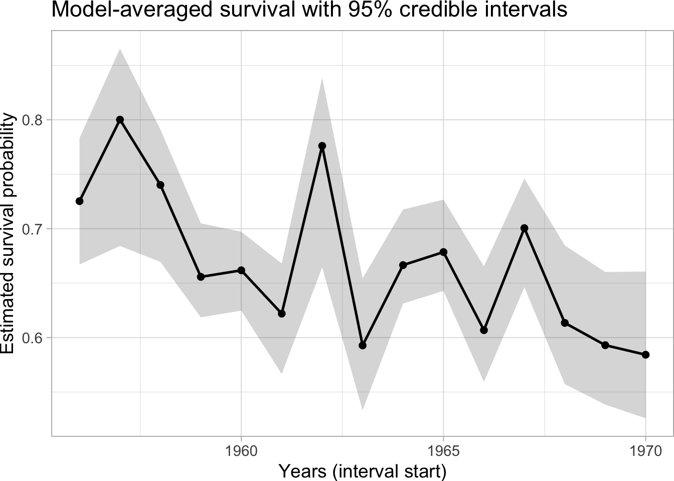
Shaded ribbons show 95% credible intervals; the solid line is the posterior mean of survival, which decreases over time, model-averaged over covariate inclusion.

6.3 Uncertainty in age

6.3.1 Motivation

Survival and other demographic parameters often differ between young and older animals, so if we blur age classes we can end up telling the wrong story about population dynamics. In Section 4.8.5, we incorporated age as a covariate in capture-recapture models, assuming it was perfectly known. With non-invasive genetics (Figure 4.1), though, age is not observed: a DNA profile can identify who was there, but not how old they were. If we ignore that uncertainty, survival estimates can be biased. Inspired by what we saw in Section 5.7, we will see here how HMM capture-recapture models can handle this kind of problem by treating age as a hidden state and separating it from what we actually observe in the field.

A neat example comes from Apennine brown bears in Gervasi et al. (2017; see also Gowan et al. 2021). Because you cannot age a bear from its DNA, the authors paired genetics with field information to classify detections into two broad age classes, cubs (<1 year) and adults (≥1 year). To do so, they used two criteria. First, classify a newly detected bear as a cub in that year if it was sampled at least once on the same date and site as a known adult female and they shared ≥1 allele at every locus (mother-offspring consistent). That’s the lenient criterion (P1). Second, apply a stricter criterion (P2): make the same mother–offspring call, but require two or more such co-sampling occasions with the same female, again on the same date and site each time.

Why two criteria? Because there’s a trade-off. P1 is better at catching real cubs (more sensitive) but risks misclassifying some adults as cubs; P2 is more conservative about calling ‘cub’, so it reduces false cubs but misses some true ones.

Instead of pretending these criteria are perfect, the authors model the misclassification explicitly: age is hidden, ‘cub/adult by P1/P2’ is what we observe, and their model estimates both classification accuracy and age-specific survival at the same time. That way, uncertainty is propagated into the demographic estimates rather than swept under the rug.

Here, I show how to encode that logic in an HMM with NIMBLE: define the hidden age states, write the transition (survival) and detection components, and add a classification step that links hidden age to the observed P1/P2 outcomes. We’ll also see how a small subset of known-age individuals (e.g., live-trapped or aged beforehand) anchors the classification step. The payoff is a set of age-specific survival estimates that are robust to imperfect age assignment, which is exactly what we need for sound ecological inference and management.

6.3.2 Model and NIMBLE implementation

To estimate bear survival, we have at our disposal a 12-year time series of non-invasive genetic sampling data, collected between 2003 and 2014. These data were kindly provided by Vincenzo Gervasi. To build up our model, we first define the states and observations:

States
- alive as cub (C)
- alive as adult (A)
- dead (D)/
Observations
- not detected (1)
- detected and classified as cub by both criteria (2)
- detected and classified as cub by P1 only (3)
- detected and classified as adult by both criteria (4)

Now we turn to writing our model.

We start with the vector of initial states. Unknown-age individuals enter as a mixture of cubs and adults: \[\begin{matrix} & \\ \mathbf{\delta} = \left ( \vphantom{ \begin{matrix} 12 \end{matrix} } \right . \end{matrix} \hspace{-1.2em} \begin{matrix} z_t=C & z_t=A & z_t=D \\ \hdashline \pi & 1 - \pi & 0\\ \end{matrix} \hspace{-0.2em} \begin{matrix} & \\ \left . \vphantom{ \begin{matrix} 12 \end{matrix} } \right ) \begin{matrix} \end{matrix} \end{matrix}\]

where \(\pi\) is the probability of being alive as a cub, and \(1 - \pi\) is the probability of being alive as an adult. For bears with known age at first detection, we fix the initial state accordingly. In NIMBLE we implement this with an individual-specific \(\delta_i\) using equals() to pin known ages:

# Initial state
# age[i] == 0: unknown -> use delta: pi, 1 - pi
# age[i] == 1: known cub -> force delta to [1, 0, 0]
# age[i] == 2: known adult -> force delta to [0, 1, 0]
for (i in 1:N){
  delta[1, i] <- equals(age[i], 0) * pi + equals(age[i], 1)  # Pr(C)
  delta[2, i] <- equals(age[i], 0) * (1 - pi) + equals(age[i], 2)  # Pr(A)
  delta[3, i] <- 0
}

We proceed with the transition matrix that contains the survival probabilities. A cub either survives and becomes adult next year (\(\phi_C\)), or dies; adults either survive in the same class (\(\phi_A\)) or die: \[\begin{matrix} & \\ \mathbf{\Gamma} = \left ( \vphantom{ \begin{matrix} 12 \\ 12 \\ 12 \end{matrix} } \right . \end{matrix} \hspace{-1.2em} \begin{matrix} z_t=C & z_t=A & z_t=D \\ \hdashline 0 & \phi_C & 1 - \phi_C\\ 0 & \phi_A & 1 - \phi_A\\ 0 & 0 & 1 \end{matrix} \hspace{-0.2em} \begin{matrix} & \\ \left . \vphantom{ \begin{matrix} 12 \\ 12 \\ 12 \end{matrix} } \right ) \begin{matrix} z_{t-1}=C \\ z_{t-1}=A \\ z_{t-1}=D \end{matrix} \end{matrix}\]

Following the paper, adult survival is sex-specific; cub survival is common to both sexes:

# Transition matrix
for (i in 1:N){
  gamma[1,1,i] <- 0
  gamma[1,2,i] <- phiC
  gamma[1,3,i] <- 1 - phiC
  gamma[2,1,i] <- 0
  gamma[2,2,i] <- phiA[sex[i]]   # sex-specific adult survival (1=f, 2=m)
  gamma[2,3,i] <- 1 - phiA[sex[i]]
  gamma[3,1,i] <- 0
  gamma[3,2,i] <- 0
  gamma[3,3,i] <- 1
}

Last step is about the observations, which arise in two steps: detection then classification. For the detection matrix, we need to introduce intermediate observations, say \(y'\) for not detected (1), detected as cub (2) and detected as adult (2): \[\begin{matrix} & \\ \mathbf{\Omega_1} = \left ( \vphantom{ \begin{matrix} 12 \\ 12 \\ 12 \end{matrix} } \right . \end{matrix} \hspace{-1.2em} \begin{matrix} y'_t=1 & y'_t=2 & y'_t=3 \\ \hdashline 1-p_C & p_C & 0\\ 1-p_A & 0 & 1 - p_A\\ 1 & 0 & 0 \end{matrix} \hspace{-0.2em} \begin{matrix} & \\ \left . \vphantom{ \begin{matrix} 12 \\ 12 \\ 12 \end{matrix} } \right ) \begin{matrix} z_{t}=C \\ z_{t}=A \\ z_{t}=D \end{matrix} \end{matrix}\]

where \(p_C\) is detection for cubs, and \(p_A\) that for adults. Then the classification matrix is: \[\begin{matrix} & \\ \mathbf{\Omega_2} = \left ( \vphantom{ \begin{matrix} 12 \\ 12 \\ 12\end{matrix} } \right . \end{matrix} \hspace{-1.2em} \begin{matrix} y_t=1 & y_t=2 & y_t=3 & y_t=4\\ \hdashline 1 & 0 & 0 & 0\\ 0 & \beta_{C,CC} & \beta_{C,CA} & 1 - \beta_{C,CC} - \beta_{C,CA}\\ 0 & \beta_{A,CC} & \beta_{A,CA} & 1 - \beta_{A,CC} - \beta_{A,CA}\\ \end{matrix} \hspace{-0.2em} \begin{matrix} & \\ \left . \vphantom{ \begin{matrix} 12 \\ 12 \\ 12\end{matrix} } \right ) \begin{matrix} y'_{t}=1 \\ y'_{t}=2 \\ y'_{t}=3 \end{matrix} \end{matrix}\]

where \(\beta_{C,CC}\) is the probability that, being a cub, and individual is classified as cub with both criteria, \(\beta_{C,CA}\) is the probability that, being a cub, an individual is classified as cub with P1 and as adult with P2, \(\beta_{A,CC}\) is the probability that, being an adult, an individual is classified as cub with both criteria, \(\beta_{A,CA}\) is the probability that, being an adult, an individual is classified as cub with P1 and as adult with P2.

The observation matrix is the product of the two detection and classification matrices \(\mathbf{\Omega_1} \mathbf{\Omega_2}\): \[\begin{matrix} & \\ \mathbf{\Omega} = \left ( \vphantom{ \begin{matrix} 12 \\ 12 \\ 12\end{matrix} } \right . \end{matrix} \hspace{-1.2em} \begin{matrix} y_t=1 & y_t=2 & y_t=3 & y_t=4\\ \hdashline 1-p_C & p_C \beta_{C,CC} & p_C \beta_{C,CA} & p_C (1 - \beta_{C,CC} - \beta_{C,CA})\\ 1-p_A & p_A \beta_{A,CC} & p_A \beta_{A,CA} & p_A (1 - \beta_{A,CC} - \beta_{A,CA})\\ 1 & 0 & 0 & 0\\ \end{matrix} \hspace{-0.2em} \begin{matrix} & \\ \left . \vphantom{ \begin{matrix} 12 \\ 12 \\ 12\end{matrix} } \right ) \begin{matrix} z_{t}=1 \\ z_{t}=2 \\ z_{t}=3 \end{matrix} \end{matrix}\]

In code, we write \(\mathbf{\Omega_1} \mathbf{\Omega_2}\) directly, as this is faster than doing the matrix multiplication at each MCMC iteration. For simplicity we use a single detection probability \(p\) for both ages, but you can let \(p\) vary by age/sex/year or sampling method, as in the paper:

# Observation matrix
omega[1,1] <- 1 - p
omega[1,2] <- p * betaCCC
omega[1,3] <- p * betaCCA
omega[1,4] <- p * (1 - betaCCC - betaCCA)

omega[2,1] <- 1 - p
omega[2,2] <- p * betaACC
omega[2,3] <- p * betaACA
omega[2,4] <- p * (1 - betaACC - betaACA)

omega[3,1] <- 1
omega[3,2] <- 0
omega[3,3] <- 0
omega[3,4] <- 0

At first detection, the event ‘not detected’ is impossible by construction (we condition on the first detection). We therefore use an initial observation matrix \(\mathbf{\Omega}_{\text{init}}\) with \(p\) set to 1 (not shown).

The likelihood and priors are handled as usual.

6.3.3 Results and interpretation

Here are the raw results:

##         mean   sd 2.5%  50% 97.5% Rhat n.eff
## betaACA 0.05 0.02 0.02 0.04  0.08 1.00  4114
## betaACC 0.02 0.01 0.00 0.02  0.05 1.00  4211
## betaCCA 0.57 0.12 0.33 0.58  0.79 1.00   966
## betaCCC 0.30 0.10 0.13 0.29  0.50 1.00   998
## p       0.71 0.04 0.63 0.71  0.79 1.00  3329
## phiA[1] 0.88 0.03 0.80 0.88  0.94 1.00  4195
## phiA[2] 0.82 0.06 0.69 0.82  0.92 1.00  3643
## phiC    0.53 0.13 0.28 0.53  0.78 1.00  3563
## pi      0.27 0.09 0.12 0.26  0.49 1.02  1416

which we can arrange as in Table 6.1 to compare them with the results obtained by Gervasi et al. (2017):

Table 6.1: Comparison of parameter estimates for the same HMM to account for age uncertainty: our NIMBLE fit vs. Gervasi et al. (2017, Table 3). Intervals are 95% credible intervals for NIMBLE and confidence intervals for Gervasi et al.. Detection in Gervasi et al. varies by design/year; I report their overall average.
Parameter	NIMBLE	Gervasi et al. (2017)
\(\phi_C\) (cub survival)	0.53 (0.28–0.78)	0.51 (0.22–0.79)
\(\phi_{A,f}\) (adult female)	0.88 (0.80–0.94)	0.92 (0.87–0.95)
\(\phi_{A,m}\) (adult male)	0.82 (0.69–0.92)	0.85 (0.76–0.91)
\(p\) (detection)	0.71 (0.63–0.79)	≈0.71 (0.62–0.79)
\(\pi\) (cub at first detection)	0.27 (0.12–0.49)	0.062 (0.007–0.396)
\(C_{c,cc}\) (cub by both \| cub)	0.30 (0.13–0.50)	0.40 (0.15–0.72)
\(C_{c,ca}\) (cub by P1 only \| cub)	0.57 (0.33–0.79)	0.60 (0.28–0.85)
\(C_{a,cc}\) (cub by both \| adult)	0.02 (0.00–0.05)	0.067 (0.024–0.174)
\(C_{a,ca}\) (cub by P1 only \| adult)	0.05 (0.02–0.08)	0.191 (0.110–0.309)

Our NIMBLE fit reproduces the main biological signals reported for the Apennine brown bear. Survival shows the expected ordering, that cubs << adults, and adult females > adult males – with estimates that closely match the published analysis. The credible/confidence intervals overlap broadly, indicating good agreement.

Our detection estimate aligns with the study’s average detection, even though their analysis lets detection vary by design and year rather than assuming a single constant value.

For age classification (linking the hidden age to P1/P2 outcomes), mapping our parameters to theirs, we found lower adult-as-cub misclassification than the paper (and thus a higher probability that detected adults are correctly called ‘adult by both’), which still matches their qualitative take: the stricter criterion (P2) performs very well for adults.

The main divergence is in the initial state mix. Intervals overlap, but the means differ. A likely explanation is model structure: we used a single, constant detection probability, while the published analysis allows detection to vary by sampling design and year – and detectability does vary meaningfully across methods and years. Collapsing this heterogeneity into one \(p\) can nudge the mixture at first detection toward a higher cub fraction to explain patterns that the richer detection model attributes to design/year effects.

In conclusion, we managed to recover the core findings of the published study (age- and sex-specific survival and average detection). Small discrepancies appear mainly in adult misclassification rates and \(\pi\). To mirror Gervasi et al. (2017) even more closely, the natural next step is to let \(p\) vary by sampling design/year (an information I did not have), as in their best supported model.

6.4 Uncertainty in sex

6.4.1 Motivation

Many species show sex differences in demographic parameters, so mislabeling sex or discarding uncertain cases can bias the very patterns we want to estimate. In monomorphic birds for example, field sexing relies on behaviour (e.g., copulation posture, courtship displays, relative body size), and those clues vary in reliability; in the Audouin’s gull (Larus audouinii) study that motivates this section, almost 80% of individuals were never sexed in the field, making ‘known-sex only’ analyses both wasteful and biased toward higher survival.

Pradel et al. (2008; see also Genovart, Pradel, and Oro 2012) turned this problem into a HMM inference task: treat sex as a hidden state (male/female/dead) and model the sex-assignment process itself. The model developed by Pradel, Genovart and colleagues separates (i) the probability of attempting a sex judgment (with a time trend, because sexing effort increased) from (ii) criterion-specific accuracy for four behavioural clues (copulation, courtship feeding, begging for food, body size).

In brief, the message is: when field classifications are uncertain, exploit them rather than filter them out, and use HMM to couple biological states to imperfect observations and propagate classification uncertainty into survival.

That philosophy mirrors the age-uncertainty Section 6.3 we just completed: there, age was hidden and P1/P2 provided noisy age labels; here, sex is hidden and multiple behavioural criteria provide noisy sex labels.

6.4.2 Model and NIMBLE implementation

To estimate Audouin’s gull survival, we have at our disposal a dataset with 4093 marked birds from a colony at the Ebro Delta (Spain), collected over 10 years. These data were kindly provided by Meritxell Genovart and Roger Pradel. To build up our model, we first define the states and observations:

States
- alive as male (M)
- alive as female (F)
- dead (D)
Observations
- not seen (1)
- judged from copulation to be male (2)
- judged from begging food to be male (3)
- judged from coutship feeding to be male (4)
- judged from body size to be male (5)
- judged from copulation to be female (6)
- judged from begging food to be female (7)
- judged from coutship feeding to be female (8)
- judged from body size to be female (9)
- not judged (10)

Now we turn to writing our model.

We start with the vector of initial states. Unknown-sex individuals enter as a mixture of males and females with probabilities \(\pi\) and \(1-\pi\): \[\begin{matrix} & \\ \mathbf{\delta} = \left ( \vphantom{ \begin{matrix} 12 \end{matrix} } \right . \end{matrix} \hspace{-1.2em} \begin{matrix} z_t=M & z_t=F & z_t=D \\ \hdashline \pi & 1 - \pi & 0\\ \end{matrix} \hspace{-0.2em} \begin{matrix} & \\ \left . \vphantom{ \begin{matrix} 12 \end{matrix} } \right ) \begin{matrix} \end{matrix} \end{matrix}\]

We proceed with the transition matrix that contains the survival probabilities. A male either survives next year as a male (\(\phi_M\)), or dies; the same happens for females (with probability \(\phi_F\)): \[\begin{matrix} & \\ \mathbf{\Gamma} = \left ( \vphantom{ \begin{matrix} 12 \\ 12 \\ 12 \end{matrix} } \right . \end{matrix} \hspace{-1.2em} \begin{matrix} z_t=M & z_t=F & z_t=D \\ \hdashline \phi_M & 0 & 1 - \phi_M\\ 0 & \phi_F & 1 - \phi_F\\ 0 & 0 & 1 \end{matrix} \hspace{-0.2em} \begin{matrix} & \\ \left . \vphantom{ \begin{matrix} 12 \\ 12 \\ 12 \end{matrix} } \right ) \begin{matrix} z_{t-1}=M \\ z_{t-1}=F \\ z_{t-1}=D \end{matrix} \end{matrix}\]

The vector of initial states and the matrix of transition probabilities are written as usual in NIMBLE:

  delta[1] <- pi
  delta[2] <- 1 - pi
  delta[3] <- 0
  
  gamma[1,1] <- phiM            
  gamma[1,2] <- 0               
  gamma[1,3] <- 1 - phiM        
  gamma[2,1] <- 0               
  gamma[2,2] <- phiF            
  gamma[2,3] <- 1 - phiF        
  gamma[3,1] <- 0               
  gamma[3,2] <- 0               
  gamma[3,3] <- 1

Last step is the observation matrix, which we write as follows (its transposed for convenience): \[\begin{matrix} & \\ \mathbf{\Omega'} = \left ( \vphantom{ \begin{matrix} 12 \\ 12 \\ 12 \\ 12 \\ 12 \\ 12 \\ 12 \\ 12 \\ 12 \\ 12 \end{matrix} } \right . \end{matrix} \hspace{-1.2em} \begin{matrix} z_t=M & z_t=F & z_t=D \\ \hdashline 1 - p & 1 - p & 1\\ p e (1-m_4) m_1 x_1 & p e (1-m_4) m_1 (1-x_1) & 0\\ p e (1-m_4) m_2 x_2 & p e (1-m_4) m_2 (1-x_2) & 0\\ p e (1-m_4) m_3 x_3 & p e (1-m_4) m_3 (1-x_3) & 0\\ p e m_4 x_4 & p e m_4 (1-x_4) & 0\\ p e (1-m_4) m_1 (1-x_1) & p e (1-m_4) m_1 x_1 & 0\\ p e (1-m_4) m_2 (1-x_2) & p e (1-m_4) m_2 x_2 & 0\\ p e (1-m_4) m_3 (1-x_3) & p e (1-m_4) m_3 x_3 & 0\\ p e m_4 (1-x_4) & p e m_4 x_4 & 0\\ p (1-e) & p (1-e) & 0\\ \end{matrix} \hspace{-0.2em} \begin{matrix} & \\ \left . \vphantom{ \begin{matrix} 12 \\ 12 \\ 12 \\ 12 \\ 12 \\ 12 \\ 12 \\ 12 \\ 12 \\ 12\end{matrix} } \right ) \begin{matrix} y_{t}=1 \\ y_{t}=2 \\ y_{t}=3 \\ y_{t}=4 \\ y_{t}=5 \\ y_{t}=6 \\ y_{t}=7 \\ y_{t}=8 \\ y_{t}=9 \\ y_{t}=10 \end{matrix} \end{matrix}\]

This matrix is a bit more complex than what we have encountered before, and needs some explanations. When an individual is encountered (with probability \(p\)), there is some chance that it will be sexed (\(e\)) based on its general appearance (body size: probability \(m_4\)) or its behaviour (probability \(1 - m_4\)). When behaviour is used, there are three different criteria (copulation, begging for food and courtship feeding), which occur with probabilities \(m_1\), \(m_2\), and \(m_3\), respectively. Finally, each criterion has its own reliability (probabilities \(x_1\), \(x_2\), \(x_3\), \(x_4\), where \(x_4\) is the reliability of the body-size criterion).

I admit that this matrix representation can be difficult to grasp at once. It can be easier to split the observation matrix in several steps, like encountering, sexing, body size sexing, sex determination and correctness, then to sketch a decision tree as in Figure 2 of Genovart, Pradel, and Oro (2012) (see also appendix S1 in that same paper).

In code, this gives:

omega[1,1] <- 1 - p                                  
omega[1,2] <- p * e * (1 - m[4]) * m[1] * x[1]      
omega[1,3] <- p * e * (1 - m[4]) * m[2] * x[2]      
omega[1,4] <- p * e * (1 - m[4]) * m[3] * x[3]      
omega[1,5] <- p * e * m[4] * x[4]      
omega[1,6] <- p * e * (1 - m[4]) * m[1] * (1 - x[1])      
omega[1,7] <- p * e * (1 - m[4]) * m[2] * (1 - x[2])      
omega[1,8] <- p * e * (1 - m[4]) * m[3] * (1 - x[3])      
omega[1,9] <- p * e * m[4] * (1 - x[4])      
omega[1,10] <- p * (1 - e)      

omega[2,1] <- 1 - p                                  
omega[2,2] <- p * e * (1 - m[4]) * m[1] * (1 - x[1])      
omega[2,3] <- p * e * (1 - m[4]) * m[2] * (1 - x[2])      
omega[2,4] <- p * e * (1 - m[4]) * m[3] * (1 - x[3])      
omega[2,5] <- p * e * m[4] * (1 - x[4])      
omega[2,6] <- p * e * (1 - m[4]) * m[1] * x[1]      
omega[2,7] <- p * e * (1 - m[4]) * m[2] * x[2]     
omega[2,8] <- p * e * (1 - m[4]) * m[3] * x[3]   
omega[2,9] <- p * e * m[4] * x[4]   
omega[2,10] <- p * (1 - e)      

omega[3,1] <- 1                                  
omega[3,2] <- 0     
omega[3,3] <- 0     
omega[3,4] <- 0     
omega[3,5] <- 0     
omega[3,6] <- 0     
omega[3,7] <- 0     
omega[3,8] <- 0     
omega[3,9] <- 0     
omega[3,10] <- 0

At first detection, the observation ‘not detected’ is impossible by construction (we condition on the first detection). We therefore use an initial observation matrix \(\mathbf{\Omega}_{\text{init}}\) with \(p\) set to 1 (not shown).

The likelihood and priors are handled as usual.

6.4.3 Results and interpretation

Here are the raw results:

##      mean   sd 2.5%  50% 97.5% Rhat n.eff
## e    0.07 0.00 0.07 0.07  0.07 1.01   589
## m[1] 0.29 0.02 0.26 0.29  0.32 1.00   913
## m[2] 0.60 0.02 0.56 0.60  0.63 1.00   892
## m[3] 0.11 0.01 0.09 0.11  0.14 1.00   817
## m[4] 0.17 0.01 0.14 0.17  0.19 1.01   949
## p    0.65 0.00 0.64 0.65  0.66 1.00   394
## phiF 0.90 0.01 0.89 0.90  0.91 1.01   205
## phiM 0.89 0.01 0.88 0.89  0.90 1.01   279
## pi   0.52 0.01 0.50 0.52  0.55 1.00   291
## x[1] 0.52 0.03 0.45 0.52  0.58 1.01   915
## x[2] 0.55 0.02 0.50 0.55  0.60 1.01   725
## x[3] 0.54 0.05 0.44 0.55  0.65 1.00   927
## x[4] 0.58 0.04 0.50 0.58  0.67 1.00   753

which we can arrange in as in Table 6.2 to compare them with the results obtained by Pradel et al. (2008):

Table 6.2: Comparison of parameter estimates for the same HMM to account for sex uncertainty: our NIMBLE fit vs. Pradel et al. (2008, Table 5, model B no genetically sexed anchors). Intervals are 95% credible intervals for NIMBLE and confidence intervals for Pradel et al.. Our error rates are 1 − x[i]. Pradel’s m’s were provided by the main author of the paper himself. Note that m4 is time-varying; the estimates were for t=1,…,10: 0.001, 0.002, 0.004, 0.007, 0.014, 0.026, 0.047, 0.084, 0.146, 0.242.
Parameter	NIMBLE	Pradel et al. (2008)
\(\mu\) (proportion male)	0.52 (0.50–0.55)	0.53 (SE 0.03)
\(\phi_F\) (female survival)	0.90 (0.89–0.91)	0.91 (SE 0.01)
\(\phi_M\) (male survival)	0.89 (0.88–0.90)	0.86 (SE 0.01)
\(m_1\) (Copulation)	0.29 (0.26–0.32)	0.29
\(m_2\) (Begging)	0.60 (0.56–0.63)	0.60
\(m_3\) (Courtship feeding)	0.11 (0.09–0.14)	0.11
\(m_4\) (Body size)	0.17 (0.14–0.19)	time-varying (see caption)
Error (Copulation)	0.48 (0.42–0.55)	0.06 (SE 0.04)
Error (Begging)	0.45 (0.40–0.50)	0.06 (SE 0.03)
Error (Courtship feeding)	0.46 (0.35–0.56)	0.00 (SE 0.16)
Error (Body size)	0.42 (0.33–0.50)	0.09 (SE 0.07)

Our NIMBLE fit recovers the main biological signals reported for the Audouin’s gulls analysis. Survival shows the expected ordering – adult females ≥ adult males – with broadly overlapping intervals and means that are close to the published model. In our run, the female–male gap is a bit smaller (0.90 vs 0.89), but the direction matches the paper’s message (higher female survival).

We used a single, constant detection probability and obtained \(p \approx 0.65\), which sits near the middle of the year‐specific values obtained by the authors (not shown in the paper).

The estimated probabilities of which clue is used align closely with the published analysis for the three ‘behavioural’ criteria: \(m_1 \approx 0.29\) (copulation), \(m_2 \approx 0.60\) (begging), \(m_3 \approx 0.11\) (courtship feeding). The paper lets body size use vary over time; our constant estimate (\(m_4 \approx 0.17\)) should be read as a pooled average across years—consistent with their finding of a low but increasing use of this criterion.

The main discrepancy lies in the error rates by criterion. The published analysis finds low misclassification (roughly 5–10% for most criteria, with a very imprecise estimate for courtship feeding). Our fit suggests substantially higher error across criteria. That discrepancy is where we expect sensitivity when there are no known‐sex anchors (and some components are simplified). Without anchors, the model can admit dual solutions (swapping sex labels and flipping error probabilities) that fit nearly equally well; small modelling choices or initial values can tip the chain toward one mode, see Pradel et al. (2008).

Our estimate of the proportion of males at first encounter (\(\mu \approx 0.52\)) agrees closely with the published result, reinforcing that the state mix is well constrained by the data even when sex is uncertain.

To conclude, the sex‐uncertainty HMM retrieves the core demographic pattern (female ≥ male survival) and matches the paper on overall detectability and the use of criteria. To mirror the published results more closely, one could add a small anchor set of genetically sexed individuals (an information used in Pradel et al. 2008 but that I did not have).

Introduction

7 Addressing model lack of fit