4 Alive and dead
4.1 Introduction
In this fourth chapter, you will learn about the Cormack-Jolly-Seber model that allows estimating survival based on capture-recapture data. You will also see how to deal with covariates to try and explain temporal and/or individual variation in survival. This chapter will also be the opportunity to introduce tools to compare models and assess their quality of fit to data.
4.2 The Cormack-Jolly-Seber (CJS) model
In Chapter 3, we introduced a capture-recapture model with constant survival and detection probabilities which we formulated as a HMM and fitted to data in NIMBLE. Historically, however, it was a slightly more complicated model that was first proposed – the so-called Cormack-Jolly-Seber (CJS) model – in which survival and recapture probabilities are time-varying. This feature of the CJS model is useful to account for variation due to environmental conditions in survival or to sampling effort in detection. Schematically the CJS model can be represented this way:
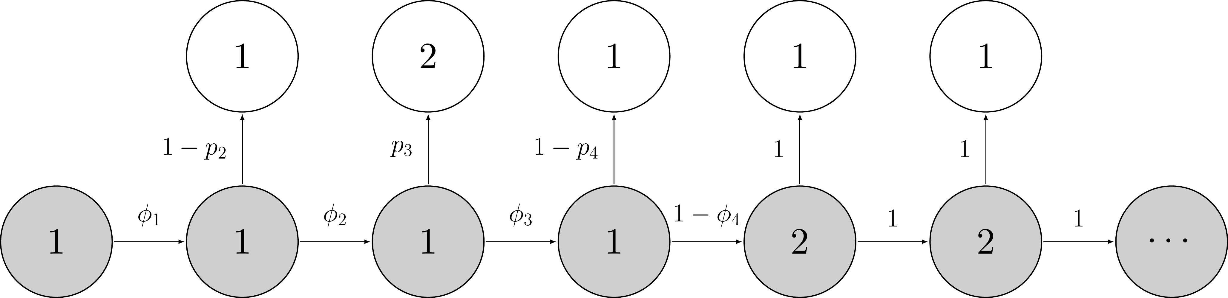
Note that the states (in gray) and the observations (in white) do not change. We still have \(z = 1\) for alive, \(z = 2\) for dead, \(y = 1\) for non-detected, and \(y = 2\) for detected.
Parameters are now indexed by time. The survival probability is defined as the probability of staying alive (or “ah, ha, ha, ha, stayin’ alive” like the Bee Gees would say) over the interval between \(t\) and \(t+1\), that is \(\phi_t = \Pr(z_{t+1} = 1 | z_t = 1)\). The detection probability is defined as the probability of being observed at \(t\) given you’re alive at \(t\), that is \(p_t = \Pr(y_{t} = 1 | z_t = 1)\). It is important to bear in mind for later (see Section 4.8) that survival operates over an interval while detection occurs at a specific time.
The CJS model is named after the three statisticians – Richard Cormack, George Jolly and George Seber – who each published independently a paper introducing more or less the same approach, a year apart ! In fact, Richard Cormack and George Jolly were working in the same corridor in Scotland back in the 1960’s. They would meet every day at coffee and would play some game together, but never mention work and were not aware of each other’s work.
4.3 Capture-recapture data
Before we turn to fitting the CJS model to actual data, let’s talk about capture-recapture for a minute. We said in Section 3.6.1 that animals are individually marked. This can be accomplished in two ways, either with artificial marks like rings for birds or ear tags for mammals, or (non-invasive) natural marks like coat patterns or feces DNA sequencing (Figure 4.1).
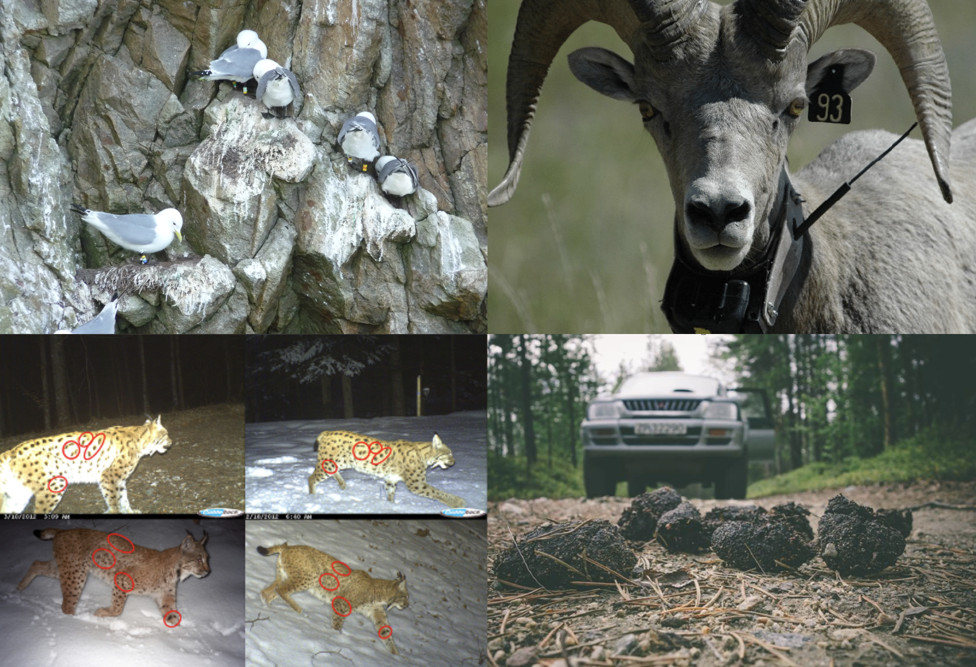
Figure 4.1: Animal individual marking. Top-left: rings (credit: Emannuelle Cam and Jean-Yves Monat); Top-right: ear-tags (credit: Kelly Powell); Bottom left: coat patterns (credit: Fridolin Zimmermann); Bottom right: ADN feces (credit: Alexander Kopatz)
Throughout this chapter, we will use data on the White-throated Dipper (Cinclus cinclus; dipper hereafter) kindly provided by Gilbert Marzolin (Figure 4.2). In total, 294 dippers with known sex and wing length were captured and recaptured between 1981 and 1987 during the March-June period. Birds were at least 1 year old when initially banded.
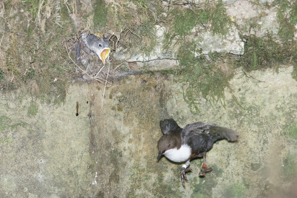
Figure 4.2: White-throated Dipper (Cinclus cinclus). Credit: Gilbert Marzolin.
The data look like:
dipper <- read_csv("dipper.csv")
dipper
## # A tibble: 294 × 9
## year_1981 year_1982 year_1983 year_1984 year_1985
## <dbl> <dbl> <dbl> <dbl> <dbl>
## 1 1 1 1 1 1
## 2 1 1 1 1 1
## 3 1 1 1 1 0
## 4 1 1 1 1 0
## 5 1 1 0 1 1
## 6 1 1 0 0 0
## 7 1 1 0 0 0
## 8 1 1 0 0 0
## 9 1 1 0 0 0
## 10 1 1 0 0 0
## # ℹ 284 more rows
## # ℹ 4 more variables: year_1986 <dbl>, year_1987 <dbl>,
## # sex <chr>, wing_length <dbl>The first seven columns are years in which Gilbert went on the field and captured the birds. A 0 stands for a non-detection, and a 1 for a detection. The eighth column informs on the sex of the bird, with F for female and M for male. The last column gives a measure wing length the first time a bird was captured.
4.4 Fitting the CJS model to the dipper data with NIMBLE
To write the NIMBLE code corresponding to the CJS model, we only need to make a few adjustments to the NIMBLE code for the model with constant parameters from Section 3.7. The main modification concerns the observation and transition matrices which we need to make time-varying. These matrices therefore become arrays and inherit a third dimension for time, besides that for rows and columns. Also we need priors for all time-varying survival phi[t] ~ dunif(0, 1) and detection p[t] ~ dunif(0, 1) probabilities. We write:
...
# parameters
  delta[1] <- 1                 # Pr(alive t = 1) = 1
  delta[2] <- 0                 # Pr(dead t = 1) = 0
  for (t in 1:(T-1)){
    phi[t] ~ dunif(0, 1)        # prior survival
    gamma[1,1,t] <- phi[t]      # Pr(alive t -> alive t+1)
    gamma[1,2,t] <- 1 - phi[t]  # Pr(alive t -> dead t+1)
    gamma[2,1,t] <- 0           # Pr(dead t -> alive t+1)
    gamma[2,2,t] <- 1           # Pr(dead t -> dead t+1)
    p[t] ~ dunif(0, 1)          # prior detection
    omega[1,1,t] <- 1 - p[t]    # Pr(alive t -> non-detected t)
    omega[1,2,t] <- p[t]        # Pr(alive t -> detected t)
    omega[2,1,t] <- 1           # Pr(dead t -> non-detected t)
    omega[2,2,t] <- 0           # Pr(dead t -> detected t)
  }
...
The likelihood does not change, except that the time-varying observation and transition matrices need to be used appropriately. Also, because we now deal with several cohorts of animals first captured, marked and released each year (in contrast with a single cohort as in Chapter 3), we need to start the loop over time from the first capture for each individual. Therefore, we write:
...
# likelihood
  for (i in 1:N){
    z[i,first[i]] ~ dcat(delta[1:2])
    for (j in (first[i]+1):T){
      z[i,j] ~ dcat(gamma[z[i,j-1], 1:2, j-1])
      y[i,j] ~ dcat(omega[z[i,j], 1:2, j-1])
    }
  }
...
At first capture, all individuals are alive z[i,first[i]] ~ dcat(delta[1:2]) and detection is 1, then after first capture for (j in (first[i]+1):T) we apply the transition and observation matrices.
Overall, the code looks like:
hmm.phitpt <- nimbleCode({
  # parameters
  delta[1] <- 1                 # Pr(alive t = 1) = 1
  delta[2] <- 0                 # Pr(dead t = 1) = 0
  for (t in 1:(T-1)){
    phi[t] ~ dunif(0, 1)        # prior survival
    gamma[1,1,t] <- phi[t]      # Pr(alive t -> alive t+1)
    gamma[1,2,t] <- 1 - phi[t]  # Pr(alive t -> dead t+1)
    gamma[2,1,t] <- 0           # Pr(dead t -> alive t+1)
    gamma[2,2,t] <- 1           # Pr(dead t -> dead t+1)
    p[t] ~ dunif(0, 1)          # prior detection
    omega[1,1,t] <- 1 - p[t]    # Pr(alive t -> non-detected t)
    omega[1,2,t] <- p[t]        # Pr(alive t -> detected t)
    omega[2,1,t] <- 1           # Pr(dead t -> non-detected t)
    omega[2,2,t] <- 0           # Pr(dead t -> detected t)
  }
  # likelihood
  for (i in 1:N){
    z[i,first[i]] ~ dcat(delta[1:2])
    for (j in (first[i]+1):T){
      z[i,j] ~ dcat(gamma[z[i,j-1], 1:2, j-1])
      y[i,j] ~ dcat(omega[z[i,j], 1:2, j-1])
    }
  }
})
We extract the detections and non-detections from the data:
We get the occasion of first capture for all individuals, by finding the position of detections in the encounter history (which(x !=0)), and keeping the first one:
Now we specify the constants:
my.constants <- list(N = nrow(y), # number of animals
T = ncol(y), # number of sampling occasions
first = first) # first capture for all animalesWe then put the data in a list. We add 1 to the data to code non-detections as 1’s detections as 2’s (see Section 3.7).
my.data <- list(y = y + 1)Let’s write a function for the initial values. For the latent states, we go the easy way, and say that all individuals are alive through the study period:
zinits <- y + 1 # non-detection -> alive
zinits[zinits == 2] <- 1 # dead -> alive
initial.values <- function() list(phi = runif(my.constants$T-1,0,1),
p = runif(my.constants$T-1,0,1),
z = zinits)We specify the parameters we would like to monitor, survival and detection probabilities here:
parameters.to.save <- c("phi", "p")We provide MCMC details:
n.iter <- 5000
n.burnin <- 1000
n.chains <- 2And we run NIMBLE:
mcmc.phitpt <- nimbleMCMC(code = hmm.phitpt,
constants = my.constants,
data = my.data,
inits = initial.values,
monitors = parameters.to.save,
niter = n.iter,
nburnin = n.burnin,
nchains = n.chains)We may have a look to the numerical summaries:
MCMCsummary(mcmc.phitpt, params = c("phi","p"), round = 2)
## mean sd 2.5% 50% 97.5% Rhat n.eff
## phi[1] 0.72 0.13 0.45 0.72 0.96 1.00 553
## phi[2] 0.45 0.07 0.32 0.45 0.60 1.01 1175
## phi[3] 0.48 0.06 0.36 0.48 0.60 1.00 1320
## phi[4] 0.63 0.06 0.51 0.63 0.75 1.01 1041
## phi[5] 0.60 0.06 0.49 0.60 0.71 1.01 1030
## phi[6] 0.70 0.14 0.49 0.69 0.97 1.00 86
## p[1] 0.67 0.13 0.39 0.67 0.90 1.00 923
## p[2] 0.87 0.08 0.68 0.88 0.98 1.00 690
## p[3] 0.88 0.06 0.73 0.89 0.97 1.00 840
## p[4] 0.88 0.06 0.75 0.89 0.96 1.02 860
## p[5] 0.90 0.05 0.79 0.91 0.98 1.01 740
## p[6] 0.76 0.14 0.51 0.77 0.98 1.00 95There is not so much time variation in the detection probability which is estimated high around 0.90. Note that p[1] corresponds to the detection probability in 1982 that is \(p_2\), p[2] to detection in 1983 therefore \(p_3\), and so on. The dippers seem to have experienced a decrease in survival in years 1982-1983 (phi[2]) and 1983-1984 (phi[4]). We will get back to that in Section 4.8.
You may have noticed the small effective sample size for the last survival (phi[6]) and detection (p[6]) probabilities. Let’s have a look to mixing for parameter phi[6] for example:
priors <- runif(3000, 0, 1)
MCMCtrace(object = mcmc.phitpt,
ISB = FALSE,
exact = TRUE,
params = c("phi[6]"),
pdf = FALSE,
priors = priors)
Clearly mixing (left panel in the plot above) is bad and there is a big overlap between the prior and the posterior for this parameter (right panel) suggesting that its prior was not well updated with the data. What is going on? If you could inspect the likelihood of the CJS model, you would realize that these two parameters \(\phi_6\) and \(p_7\) appear only as the product \(\phi_6 p_7\) and cannot be estimated separately. In other words, one of these parameters is redundant, and you’d need an extra sampling occasion to be able to disentangle them. This is not a big issue as long as you’re aware of it and you do not attempt to ecologically interpret these parameters.
4.5 CJS model derivatives
Besides the model we considered with constant parameters (see Chapter 3) and the CJS model with time-varying parameters, you might want to fit in-between or models with time variation on either detection or survival.
But I realize that we did not actually fit the model with constant parameters from Chapter 3. Let’s do it. You should be familiar with the process by now:
# NIMBLE code
hmm.phip <- nimbleCode({
phi ~ dunif(0, 1) # prior survival
p ~ dunif(0, 1) # prior detection
# likelihood
gamma[1,1] <- phi # Pr(alive t -> alive t+1)
gamma[1,2] <- 1 - phi # Pr(alive t -> dead t+1)
gamma[2,1] <- 0 # Pr(dead t -> alive t+1)
gamma[2,2] <- 1 # Pr(dead t -> dead t+1)
delta[1] <- 1 # Pr(alive t = 1) = 1
delta[2] <- 0 # Pr(dead t = 1) = 0
omega[1,1] <- 1 - p # Pr(alive t -> non-detected t)
omega[1,2] <- p # Pr(alive t -> detected t)
omega[2,1] <- 1 # Pr(dead t -> non-detected t)
omega[2,2] <- 0 # Pr(dead t -> detected t)
for (i in 1:N){
z[i,first[i]] ~ dcat(delta[1:2])
for (j in (first[i]+1):T){
z[i,j] ~ dcat(gamma[z[i,j-1], 1:2])
y[i,j] ~ dcat(omega[z[i,j], 1:2])
}
}
})
# occasions of first capture
first <- apply(y, 1, function(x) min(which(x !=0)))
# constants
my.constants <- list(N = nrow(y),
T = ncol(y),
first = first)
# data
my.data <- list(y = y + 1)
# initial values
zinits <- y + 1 # non-detection -> alive
zinits[zinits == 2] <- 1 # dead -> alive
initial.values <- function() list(phi = runif(1,0,1),
p = runif(1,0,1),
z = zinits)
# parameters to monitor
parameters.to.save <- c("phi", "p")
# MCMC details
n.iter <- 5000
n.burnin <- 1000
n.chains <- 2
# run NIMBLE
mcmc.phip <- nimbleMCMC(code = hmm.phip,
constants = my.constants,
data = my.data,
inits = initial.values,
monitors = parameters.to.save,
niter = n.iter,
nburnin = n.burnin,
nchains = n.chains)
## |-------------|-------------|-------------|-------------|
## |-------------------------------------------------------|
## |-------------|-------------|-------------|-------------|
## |-------------------------------------------------------|
# numerical summaries
MCMCsummary(mcmc.phip, round = 2)
## mean sd 2.5% 50% 97.5% Rhat n.eff
## p 0.90 0.03 0.83 0.90 0.94 1.00 661
## phi 0.56 0.02 0.51 0.56 0.61 1.01 1633Let’s now turn to the model with time-varying survival and constant detection. We modify the CJS model NIMBLE code by no longer having the observation matrix time-specific. I’m just providing the model code to save space:
hmm.phitp <- nimbleCode({
for (t in 1:(T-1)){
phi[t] ~ dunif(0, 1) # prior survival
gamma[1,1,t] <- phi[t] # Pr(alive t -> alive t+1)
gamma[1,2,t] <- 1 - phi[t] # Pr(alive t -> dead t+1)
gamma[2,1,t] <- 0 # Pr(dead t -> alive t+1)
gamma[2,2,t] <- 1 # Pr(dead t -> dead t+1)
}
p ~ dunif(0, 1) # prior detection
delta[1] <- 1 # Pr(alive t = 1) = 1
delta[2] <- 0 # Pr(dead t = 1) = 0
omega[1,1] <- 1 - p # Pr(alive t -> non-detected t)
omega[1,2] <- p # Pr(alive t -> detected t)
omega[2,1] <- 1 # Pr(dead t -> non-detected t)
omega[2,2] <- 0 # Pr(dead t -> detected t)
# likelihood
for (i in 1:N){
z[i,first[i]] ~ dcat(delta[1:2])
for (j in (first[i]+1):T){
z[i,j] ~ dcat(gamma[z[i,j-1], 1:2, j-1])
y[i,j] ~ dcat(omega[z[i,j], 1:2])
}
}
})We obtain the following numerical summaries for parameters, confirming high detection and temporal variation in survival:
## mean sd 2.5% 50% 97.5% Rhat n.eff
## phi[1] 0.63 0.11 0.41 0.63 0.84 1 1407
## phi[2] 0.46 0.07 0.33 0.46 0.60 1 1350
## phi[3] 0.48 0.06 0.37 0.48 0.59 1 1586
## phi[4] 0.62 0.06 0.51 0.62 0.73 1 1528
## phi[5] 0.61 0.06 0.50 0.61 0.71 1 1463
## phi[6] 0.59 0.06 0.48 0.59 0.71 1 1101
## p 0.89 0.03 0.82 0.89 0.94 1 595Now the model with time-varying detection and constant survival, for which the NIMBLE code has a constant over time transition matrix:
hmm.phipt <- nimbleCode({
phi ~ dunif(0, 1) # prior survival
gamma[1,1] <- phi # Pr(alive t -> alive t+1)
gamma[1,2] <- 1 - phi # Pr(alive t -> dead t+1)
gamma[2,1] <- 0 # Pr(dead t -> alive t+1)
gamma[2,2] <- 1 # Pr(dead t -> dead t+1)
delta[1] <- 1 # Pr(alive t = 1) = 1
delta[2] <- 0 # Pr(dead t = 1) = 0
for (t in 1:(T-1)){
p[t] ~ dunif(0, 1) # prior detection
omega[1,1,t] <- 1 - p[t] # Pr(alive t -> non-detected t)
omega[1,2,t] <- p[t] # Pr(alive t -> detected t)
omega[2,1,t] <- 1 # Pr(dead t -> non-detected t)
omega[2,2,t] <- 0 # Pr(dead t -> detected t)
}
# likelihood
for (i in 1:N){
z[i,first[i]] ~ dcat(delta[1:2])
for (j in (first[i]+1):T){
z[i,j] ~ dcat(gamma[z[i,j-1], 1:2])
y[i,j] ~ dcat(omega[z[i,j], 1:2, j-1])
}
}
})Numerical summaries for the parameters are:
## mean sd 2.5% 50% 97.5% Rhat n.eff
## phi 0.56 0.03 0.51 0.56 0.61 1.00 1296
## p[1] 0.74 0.12 0.49 0.74 0.93 1.00 1369
## p[2] 0.84 0.08 0.66 0.85 0.98 1.01 744
## p[3] 0.84 0.07 0.68 0.85 0.96 1.00 722
## p[4] 0.89 0.05 0.77 0.89 0.97 1.00 962
## p[5] 0.92 0.04 0.81 0.92 0.98 1.00 1123
## p[6] 0.90 0.07 0.74 0.91 1.00 1.01 378We note that these two models do no longer have parameter redundancy issues.
Before we move to the next section, you might ask how to fit these models with nimbleEcology as in Section 3.8.3. Conveniently there are specific NIMBLE functions for the marginalized likelihood of the CJS model and its derivatives. These function are named generically dCJSxx() where the first x is for survival and the second x is for detection and x can be s for scalar or constant or v for vector or time-dependent. For example, to implement the model with constant survival and detection probabilities, you would use dCJSss():
# load nimbleEcology in case we forgot previously
library(nimbleEcology)
# data
y <- dipper %>%
  select(year_1981:year_1987) %>%
  as.matrix()
y <- y[ first != ncol(y), ] # get rid of individuals for which
# first detection = last capture
# NIMBLE code
hmm.phip.nimbleecology <- nimbleCode({
phi ~ dunif(0, 1) # survival prior
p ~ dunif(0, 1) # detection prior
# likelihood
for (i in 1:N){
y[i, first[i]:T] ~ dCJS_ss(probSurvive = phi,
probCapture = p,
len = T - first[i] + 1)
}
})
# occasions of first capture
first <- apply(y, 1, function(x) min(which(x !=0)))
# constants
my.constants <- list(N = nrow(y),
T = ncol(y),
first = first)
# data
my.data <- list(y = y) # 0 = non-detected, 1 = detected
# initial values: marginalized likelihood, hence no latent states
# therefore no need for initial values for latent states
initial.values <- function() list(phi = runif(1,0,1),
p = runif(1,0,1))
# parameters to monitor
parameters.to.save <- c("phi", "p")
# MCMC details
n.iter <- 2500
n.burnin <- 1000
n.chains <- 2
# run NIMBLE
mcmc.phip.nimbleecology <- nimbleMCMC(code = hmm.phip.nimbleecology,
constants = my.constants,
data = my.data,
inits = initial.values,
monitors = parameters.to.save,
niter = n.iter,
nburnin = n.burnin,
nchains = n.chains)
## |-------------|-------------|-------------|-------------|
## |-------------------------------------------------------|
## |-------------|-------------|-------------|-------------|
## |-------------------------------------------------------|
# numerical summaries
MCMCsummary(mcmc.phip.nimbleecology, round = 2)
## mean sd 2.5% 50% 97.5% Rhat n.eff
## p 0.90 0.03 0.83 0.90 0.94 1.00 668
## phi 0.56 0.02 0.51 0.56 0.61 1.01 723We are left with four models, each saying a different story about the data, with temporal variation or not in either survival or detection probability. How to quantify the most plausible of these four ecological hypotheses? Rendez-vous in the next section.
4.6 Model comparison with WAIC
Which of the four models above is best supported by the data? To address this question, we need to remember that we used all the observed data to fit these models. What really matters is how well each model will perform when predicting future data, a property known as predictive accuracy. A natural measure of predictive accuracy is the likelihood, often referred in the context of model comparison as the predictive density. In practice, however, we do not know the true process or the future data, so the predictive density can only be estimated, and with some bias.
You may have heard about the Akaike Information Criterion (AIC) in the frequentist framework, and the Deviance Information Criterion (DIC) in the Bayesian framework. Here, we will also consider the Widely Applicable Information Criterion or Watanabe Information Criterion (WAIC). AIC, DIC and WAIC each aim to provide an approximation of predictive accuracy.
While AIC is the predictive measure of choice in the frequentist framework for ecologists, DIC has been around for some time for Bayesian applications due to its availability in popular BUGS pieces of software. However, AIC and BIC use a point estimate of the unknown parameters, while we have access to their entire (posterior) distribution with the Bayesian approach. Also, DIC has been shown to misbehave when the posterior distribution is not well summarized by its mean. For a more fully Bayesian approach we would like to use the entire posterior distribution to evaluate the predictive performance, which is exactly what WAIC does.
Conveniently, NIMBLE calculates WAIC for you. The only modification you need to make is to add WAIC = TRUE in the call to the nimbleMCMC() function. For example, for the CJS model, we write:
mcmc.phitpt <- nimbleMCMC(code = hmm.phitpt,
constants = my.constants,
data = my.data,
inits = initial.values,
monitors = parameters.to.save,
niter = n.iter,
nburnin = n.burnin,
nchains = n.chains,
WAIC = TRUE) I re-ran the four models to calculate the WAIC value for each of them
data.frame(model = c("both survival & detection constant",
"time-dependent survival, constant detection",
"constant survival, time-dependent detection",
"both survival & detection time-dependent"),
WAIC = c(mcmc.phip$WAIC$WAIC,
mcmc.phitp$WAIC$WAIC,
mcmc.phipt$WAIC$WAIC,
mcmc.phitpt$WAIC$WAIC))## model WAIC
## 1 both survival & detection constant 266.7
## 2 time-dependent survival, constant detection 273.0
## 3 constant survival, time-dependent detection 270.9
## 4 both survival & detection time-dependent 308.9Lower values of WAIC imply higher predictive accuracy, thefore we would favor model with constant parameters.
4.7 Goodness of fit
In the previous section, Section 4.6, we compared models between each other based on their predictive accuracy – we assessed their relative fit. However, even though we were able to rank these models according to predictive accuracy, it could happen that all models actually had poor predictive performance – this has to do with absolute fit.
How to assess the goodness of fit of the CJS model to capture-recapture data?
4.7.1 Posterior predictive checks
In the Bayesian framework, we use posterior predictive checks to assess absolute model fit. The basic idea is to compare the observed data with replicated data generated from the model. If the model is a good fit to the data, then the replicated data predicted from the model should look similar to the observed data. To make the comparison tractable, some summary statistics are generally used. For the CJS model, this is often done with the m-array, which records the number of individuals released in a given year and first recaptured in subsequent years. For examples, see Kéry and Schaub (2011), Paganin and de Valpine (2025), and the NIMBLE website https://r-nimble.org/examples/posterior_predictive.html.
Posterior predictive checks are powerful tools. However, there are long-established procedures for evaluating absolute fit and diagnosing violations of specific CJS model assumptions, and it would be a shame to ignore them.
4.7.2 Classical tests
We focus here on two assumptions that have an ecological interpretation: transience and trap-dependence. The transience test evaluates whether newly encountered individuals are as likely to be detected again as previously encountered ones. A signal of transience is often seen as an excess of individuals never seen again. The trap-dependence test evaluates whether individuals that were not detected at a given occasion are as likely to be detected at the next occasion as those that were. Trap-dependence is often seen as an effect of trapping on detection. Although these tests are commonly referred to as the test of transience and the test of trap-dependence, you should keep in mind that transience and trap-dependence are only two possible reasons why these tests may reveal a lack of fit.
These tests are implemented in the package R2ucare, and we illustrate its use with the dipper data.
We load the package R2ucare:
# To install the R2ucare package:
# if(!require(devtools)) install.packages("devtools")
# devtools::install_github("oliviergimenez/R2ucare")
library(R2ucare)We get the capture-recapture data:
# capture-recapture data
dipper <- read_csv("dat/dipper.csv")
# get encounter histories
y <- dipper %>%
select(year_1981:year_1987) %>%
as.matrix()
# number of birds with a particular capture-recapture history
size <- rep(1, nrow(y))We may perform a test specifically to assess a transient effect:
test3sr(y, size)
## $test3sr
## stat df p_val sign_test
## 1.773 5.000 0.880 -0.054
##
## $details
## component stat p_val signed_test test_perf
## 1 2 0.08 0.778 0.283 Chi-square
## 2 3 0.232 0.63 0.482 Chi-square
## 3 4 0.847 0.358 -0.92 Chi-square
## 4 5 0.288 0.592 -0.537 Chi-square
## 5 6 0.326 0.568 0.571 Chi-squareOr trap-dependence:
test2ct(y, size)
## $test2ct
## stat df p_val sign_test
## 9.463 4.000 0.051 -1.538
##
## $details
## component dof stat p_val signed_test test_perf
## 1 2 1 0 1 0 Fisher
## 2 3 1 0 1 0 Fisher
## 3 4 1 0 1 0 Fisher
## 4 5 1 9.463 0.002 -3.076 FisherNone of these tests is significant, but what to do if these tests are significant? Transience can occur for different reasons. Some animals may simply pass through without belonging to the study population (true transients). Others may reproduce once and then die or permanently disperse, reflecting the cost of first reproduction. In some cases, marking itself may cause individuals to die or leave the area. Whatever the cause, these transient individuals are never detected again after their initial capture, so their probability of local survival is zero after initial capture.
This suggests a way to account for transience by modeling a two-age class effect on survival, where age here refers not to biological age but to time since first capture. The first age class, Age 1, corresponds to newly marked in the interval immediately following capture. This is where transients live: if they are true transients, they will never be seen again because their local survival after marking is effectively 0. The second age class, Age 2+ corresponds to established residents and all subsequent intervals for individuals that remained in the study population beyond the first interval.
We allow survival to differ between these two ages, defining \(\phi_1\) as the apparent survival in the first interval after initial capture, and \(\phi_{2+}\) as the apparent survival in all subsequent intervals. If there are transients, \(\phi_1\) will be pulled lower than \(\phi_{2+}\), since the first interval mixes true residents (who survive locally with probability \(\phi_{2+}\)) and transients (who never survive locally to the next occasion). A useful quantity to compute here is the transient proportion \(\tau\), defined as \(\displaystyle \tau = 1 - \frac{\phi_{1}}{\phi_{2+}}\).
We will later see in Section 4.8.5 how to encode an age effect on survival, and I will use this approach I just described to account for transience in Section 7.2. Note also that transience can be represented through states in a HMM (see Genovart and Pradel 2019 for more details).
Trap-dependence may arise in several ways. It can occur when animals are directly affected by trapping, either positively or negatively (true trap-dependence). It may also result from observers visiting some parts of the study area more often after individuals have been detected (preferential sampling), or from habitat heterogeneity, where some patches are more accessible and individuals located there have higher detection probabilities (access bias). Trap-dependence can also reflect individual differences in age, sex, or social status that influence movements or activity patterns and thus detection probability (individual heterogeneity). Finally, it may arise when temporary emigration is non-random, for instance if individuals skip reproduction (skipped reproduction).
In short, trap-dependence designates some form of correlation between detection events. To address this issue, this correlation needs to be accounted for, and we show how to do so in a case study at Section 7.2.
4.7.3 Design considerations
So far, we have considered assumptions related to the model. There are also assumptions tied to the study design. In particular, when we talk about survival, it is always in reference to the study area, and we need to be clear about what this means. What we estimate is usually called apparent survival, not true survival. Apparent survival is the product of true survival and site fidelity, and is therefore always lower than true survival unless fidelity equals one.
Other design assumptions are worth noting, which I only list here. Marks should not be lost, individual identity should be recorded without error (no false positives), and captured animals should represent a random sample of the population.
4.8 Covariates
In the models we have considered so far, survival and detection probabilities may vary over time, but we do not include ecological drivers that might explain these variation. Luckily, in the spirit of generalized linear models, we can make these parameters dependent on external covariates over time, such as environmental conditions for survival or sampling effort for detection.
Besides variation over time, we will also cover individual variation in these parameters, in which for example survival vary according to sex or some phenotypic characteristics (e.g. size or body mass).
Let’s illustrate the use of covariates with the dipper example.
4.8.1 Temporal covariates
4.8.1.1 Discrete
A major flood occurred during the 1983 breeding season (from October 1982 to May 1983). Because captures during the breeding season occurred before and after the flood, survival in the two years 1982-1983 and 1983-1984 were likely to be affected. Indeed survival of a species living along and feeding in the river in these two flood years was most likely lower than in nonflood years. Here we will use a discrete or categorical covariate, or a group.
Let’s use a covariate flood that contains 1s and 2s, indicating whether we are in a flood or nonflood year for each year: 1 if nonflood year, and 2 if flood year.
flood <- c(1, # 1981-1982 (nonflood)
2, # 1982-1983 (flood)
2, # 1983-1984 (flood)
1, # 1984-1985 (nonflood)
1, # 1985-1986 (nonflood)
1) # 1986-1987 (nonflood)Then we write the model code:
hmm.phifloodp <- nimbleCode({
delta[1] <- 1 # Pr(alive t = 1) = 1
delta[2] <- 0 # Pr(dead t = 1) = 0
for (t in 1:(T-1)){
gamma[1,1,t] <- phi[flood[t]] # Pr(alive t -> alive t+1)
gamma[1,2,t] <- 1 - phi[flood[t]] # Pr(alive t -> dead t+1)
gamma[2,1,t] <- 0 # Pr(dead t -> alive t+1)
gamma[2,2,t] <- 1 # Pr(dead t -> dead t+1)
}
p ~ dunif(0, 1) # prior detection
omega[1,1] <- 1 - p # Pr(alive t -> non-detected t)
omega[1,2] <- p # Pr(alive t -> detected t)
omega[2,1] <- 1 # Pr(dead t -> non-detected t)
omega[2,2] <- 0 # Pr(dead t -> detected t)
phi[1] ~ dunif(0, 1) # prior for survival in nonflood years
phi[2] ~ dunif(0, 1) # prior for survival in flood years
# likelihood
for (i in 1:N){
z[i,first[i]] ~ dcat(delta[1:2])
for (j in (first[i]+1):T){
z[i,j] ~ dcat(gamma[z[i,j-1], 1:2, j-1])
y[i,j] ~ dcat(omega[z[i,j], 1:2])
}
}
})We use nested indexing above when specifying survival in the transition matrix. E.g. for year \(t = 2\), phi[flood[t]] gives phi[flood[2]] which will be phi[2] because flood[2] is 2 that (a flood year).
Let’s provide the constants in a list:
Now a function to generate initial values:
The parameters to be monitored:
parameters.to.save <- c("p", "phi")The MCMC details:
n.iter <- 5000
n.burnin <- 1000
n.chains <- 2We’re all set, and we run NIMBLE:
mcmc.phifloodp <- nimbleMCMC(code = hmm.phifloodp,
                             constants = my.constants,
                             data = my.data,
                             inits = initial.values,
                             monitors = parameters.to.save,
                             niter = n.iter,
                             nburnin = n.burnin,
                             nchains = n.chains)
The numerical summaries are given by:
MCMCsummary(mcmc.phifloodp, round = 2)## mean sd 2.5% 50% 97.5% Rhat n.eff
## p 0.89 0.03 0.83 0.90 0.95 1 609
## phi[1] 0.61 0.03 0.55 0.61 0.67 1 1474
## phi[2] 0.47 0.04 0.38 0.47 0.56 1 1700Having a look to the numerical summaries, we see that as expected, survival in flood years (phi[2]) is much lower than survival in non-flood years (phi[1]). You could formally test this difference by considering the difference phi[1] - phi[2]. Alternatively, this can be done afterwards and calculating the probability that this difference is positive (or phi[1] > phi[2]). Using a single chain for convenience, we do:
phi1 <- mcmc.phifloodp$chain1[,'phi[1]']
phi2 <- mcmc.phifloodp$chain1[,'phi[2]']
mean(phi1 - phi2 > 0)
## [1] 0.9952
An important point here is that we formulated an ecological hypothesis which we translated into a model. The next step would consist in calculating WAIC for this model and compare it with that of the four other model we have fitted so far (see Section 4.6).
Another method to include a discrete covariate consists in considering the effect of the difference between its levels. For example, we could consider survival in nonflood years as the reference and test the difference in survival with flood years.
To do so, we write survival as a linear function of our covariate on some scale, e.g. \(\text{logit}(\phi_t) = \beta_1 + \beta_2 \;\text{flood}_t\) where the \(\beta\)’s are regression coefficients we need to estimate (intercept \(\beta_1\) and slope \(\beta_2\)), and \(\text{logit}(x) = \log \displaystyle{\left(\frac{x}{1-x}\right)}\) is the logit function. The logit function lives between \(-\infty\) and \(+\infty\), and sends values between 0 and 1 onto the real line. For example \(\log(0.2/(1-0.2))=-1.39\), \(\log(0.5/(1-0.5))=0\) and \(\log(0.8/(1-0.8))=1.39\). Why use the logit function? Because survival is a probability bounded between 0 and 1, and if we used directly \(\phi_t = \beta_1 + \beta_2 \;\text{flood}_t\) we might end up with estimates for the regression coefficients that make survival out of bound. Therefore, we consider survival as a linear function of our covariates on the scale of the logit function, working on the real line, then back-transform using the inverse-logit (reciprocal function) to obtain survival on its natural scale. The inverse-logit function is \(\displaystyle{\text{logit}^{-1}(x) = \frac{\exp(x)}{1+\exp(x)} = \frac{1}{1+\exp(-x)}}\). The logit function is often called a link function like in generalized linear models. Other link functions exist, we’ll see an example in Section 5.4.2.
Another point of attention is the prior we will assign to regression coefficients. We no longer assign a prior to survival directly like previously, but we need to assign prior to the \(\beta\)’s which will induce some prior on survival. And sometimes, your priors on the regression coefficients are non-informative, but the prior on survival is not. Consider for example the case of a single intercept with no covariate. If you assign as a prior to this regression coefficient a normal distribution with mean 0 and large standard deviation (left figure below), which would be my first reflex, then you end up with a very informative prior on survival with a bathtub shape, putting much importance on low and high values (right figure below):
# 1000 random values from a N(0,10)
intercept <- rnorm(1000, mean = 0, sd = 10)
# plogis() is the inverse-logit function in R
survival <- plogis(intercept)
df <- data.frame(intercept = intercept, survival = survival)
plot1 <- df %>%
  ggplot(aes(x = intercept)) +
  geom_density() +
  labs(x = "prior on intercept")
plot2 <- df %>%
  ggplot(aes(x = survival)) +
  geom_density() +
  labs(x = "prior on survival")
plot1 + plot2
Now if you go for a lower standard deviation for the intercept prior (left figure below), e.g. 1.5, the prior on survival is non-informative, looking like a uniform distribution between 0 and 1 (right figure below):
set.seed(123)
# 1000 random values from a N(0,1.5)
intercept <- rnorm(1000, mean = 0, sd = 1.5)
# plogis() is the inverse-logit function in R
survival <- plogis(intercept)
df <- data.frame(intercept = intercept, survival = survival)
plot1 <- df %>%
  ggplot(aes(x = intercept)) +
  geom_density() +
  labs(x = "prior on intercept")
plot2 <- df %>%
  ggplot(aes(x = survival)) +
  geom_density() +
  labs(x = "prior on survival")
plot1 + plot2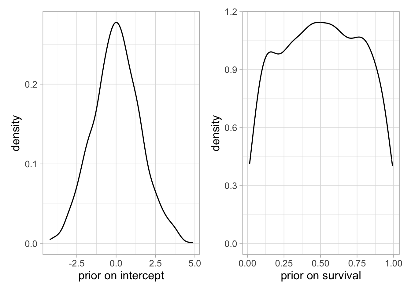
Now let’s go back to our model. We first define our flood covariate with 0 if nonflood year, and 1 if flood year:
flood <- c(0, # 1981-1982 (nonflood)
           1, # 1982-1983 (flood)
           1, # 1983-1984 (flood)
           0, # 1984-1985 (nonflood)
           0, # 1985-1986 (nonflood)
           0) # 1986-1987 (nonflood)
Then we write the NIMBLE code:
hmm.phifloodp <- nimbleCode({
  delta[1] <- 1                 # Pr(alive t = 1) = 1
  delta[2] <- 0                 # Pr(dead t = 1) = 0
  for (t in 1:(T-1)){
    logit(phi[t]) <- beta[1] + beta[2] * flood[t]
    gamma[1,1,t] <- phi[t]      # Pr(alive t -> alive t+1)
    gamma[1,2,t] <- 1 - phi[t]  # Pr(alive t -> dead t+1)
    gamma[2,1,t] <- 0           # Pr(dead t -> alive t+1)
    gamma[2,2,t] <- 1           # Pr(dead t -> dead t+1)
  }
  p ~ dunif(0, 1)               # prior detection
  omega[1,1] <- 1 - p           # Pr(alive t -> non-detected t)
  omega[1,2] <- p               # Pr(alive t -> detected t)
  omega[2,1] <- 1               # Pr(dead t -> non-detected t)
  omega[2,2] <- 0               # Pr(dead t -> detected t)
  beta[1] ~ dnorm(0, sd = 1.5)  # prior intercept
  beta[2] ~ dnorm(0, sd = 1.5)  # prior slope
  # likelihood
  for (i in 1:N){
    z[i,first[i]] ~ dcat(delta[1:2])
    for (j in (first[i]+1):T){
      z[i,j] ~ dcat(gamma[z[i,j-1], 1:2, j-1])
      y[i,j] ~ dcat(omega[z[i,j], 1:2])
    }
  }
})
We wrote \(\text{logit}(\phi_t) = \beta_1 + \beta_2 \; \text{flood}_t\), meaning that survival in nonflood years (\(\text{flood}_t = 0\)) is \(\text{logit}(\phi_t) = \beta_1\) and survival in flood years (\(\text{flood}_t = 1\)) is \(\text{logit}(\phi_t) = \beta_1 + \beta_2\). We see that \(\beta_1\) is survival in nonflood years (on the logit scale) and \(\beta_2\) is the difference between survival in flood years and survival in nonflood years (again, on the logit scale). In passing we assigned the same prior for both \(\beta_1\) and \(\beta_2\) but in certain situations, we might think twice before doing that as \(\beta_2\) is a difference between two survival probabilities (on the logit scale).
Let’s put our constants in a list:
Then our function for generating initial values:
And the parameters to be monitored:
parameters.to.save <- c("beta", "p", "phi")Finaly, we run NIMBLE:
mcmc.phifloodp <- nimbleMCMC(code = hmm.phifloodp,
                             constants = my.constants,
                             data = my.data,
                             inits = initial.values,
                             monitors = parameters.to.save,
                             niter = n.iter,
                             nburnin = n.burnin,
                             nchains = n.chains)
You may check that we get the same numerical summaries as above for survival in nonflood years (phi[1], phi[4], phi[5] and phi[6]) and flood years (phi[2] and phi[3]):
MCMCsummary(mcmc.phifloodp, round = 2)## mean sd 2.5% 50% 97.5% Rhat n.eff
## beta[1] 0.44 0.13 0.17 0.44 0.69 1.01 725
## beta[2] -0.54 0.22 -0.96 -0.54 -0.11 1.00 770
## p 0.89 0.03 0.83 0.89 0.94 1.00 631
## phi[1] 0.61 0.03 0.54 0.61 0.67 1.01 724
## phi[2] 0.47 0.04 0.39 0.47 0.56 1.00 1597
## phi[3] 0.47 0.04 0.39 0.47 0.56 1.00 1597
## phi[4] 0.61 0.03 0.54 0.61 0.67 1.01 724
## phi[5] 0.61 0.03 0.54 0.61 0.67 1.01 724
## phi[6] 0.61 0.03 0.54 0.61 0.67 1.01 724You may also check how to go from the \(\beta\)’s to the survival probabilities \(\phi\). Let’s get the draws from the posterior distribution of the \(\beta\)’s first:
beta1 <- c(mcmc.phifloodp$chain1[,'beta[1]'], # beta1 chain 1
           mcmc.phifloodp$chain2[,'beta[1]']) # beta1 chain 2
beta2 <- c(mcmc.phifloodp$chain1[,'beta[2]'], # beta2 chain 1
           mcmc.phifloodp$chain2[,'beta[2]']) # beta2 chain 2
Then apply the inverse-logit function to get survival in nonflood years, e.g. its posterior mean and credible interval:
mean(plogis(beta1))
## [1] 0.6066
quantile(plogis(beta1), probs = c(2.5, 97.5)/100)
##   2.5%  97.5%
## 0.5435 0.6651
Same thing for survival in flood years:
4.8.1.2 Continuous
Instead of a discrete covariate varying over time, we may want to consider a continuous covariate, say \(x_t\), through \(\text{logit}(\phi_t) = \beta_1 + \beta_2 x_t\). For example, let’s investigate the effect of water flow on dipper survival, which should reflect the flood that occurred during the 1983 breeding season.
We build a covariate with water flow in liters per second measured during the March to May period each year, starting with year 1982:
# water flow in L/s
water_flow <- c(443,  # March-May 1982
                1114, # March-May 1983
                529,  # March-May 1984
                434,  # March-May 1985
                627,  # March-May 1986
                466)  # March-May 1987
We do not need water flow in 1981 because we will write the probability \(\phi_t\) of being alive in year \(t + 1\) given a bird was alive in year \(t\) as a linear function of the water flow in year \(t + 1\).
You may have noticed the high value of water flow for 1983, twice as much as in the other years, corresponding to the flood. Importantly, we standardize our covariate to improve convergence:
Now we write the model code:
hmm.phiflowp <- nimbleCode({
  delta[1] <- 1                 # Pr(alive t = 1) = 1
  delta[2] <- 0                 # Pr(dead t = 1) = 0
  for (t in 1:(T-1)){
    logit(phi[t]) <- beta[1] + beta[2] * flow[t]
    gamma[1,1,t] <- phi[t]      # Pr(alive t -> alive t+1)
    gamma[1,2,t] <- 1 - phi[t]  # Pr(alive t -> dead t+1)
    gamma[2,1,t] <- 0           # Pr(dead t -> alive t+1)
    gamma[2,2,t] <- 1           # Pr(dead t -> dead t+1)
  }
  p ~ dunif(0, 1)               # prior detection
  omega[1,1] <- 1 - p           # Pr(alive t -> non-detected t)
  omega[1,2] <- p               # Pr(alive t -> detected t)
  omega[2,1] <- 1               # Pr(dead t -> non-detected t)
  omega[2,2] <- 0               # Pr(dead t -> detected t)
  beta[1] ~ dnorm(0, 1.5)       # prior intercept
  beta[2] ~ dnorm(0, 1.5)       # prior slope
  # likelihood
  for (i in 1:N){
    z[i,first[i]] ~ dcat(delta[1:2])
    for (j in (first[i]+1):T){
      z[i,j] ~ dcat(gamma[z[i,j-1], 1:2, j-1])
      y[i,j] ~ dcat(omega[z[i,j], 1:2])
    }
  }
})
We put the constants in a list:
Initial values as usual:
And parameters to be monitored:
parameters.to.save <- c("beta", "p", "phi")Eventually, we run NIMBLE:
mcmc.phiflowp <- nimbleMCMC(code = hmm.phiflowp,
                          constants = my.constants,
                          data = my.data,
                          inits = initial.values,
                          monitors = parameters.to.save,
                          niter = n.iter,
                          nburnin = n.burnin,
                          nchains = n.chains)
We can have a look to the results through a caterpillar plot of the regression parameters:
MCMCplot(object = mcmc.phiflowp, params = "beta")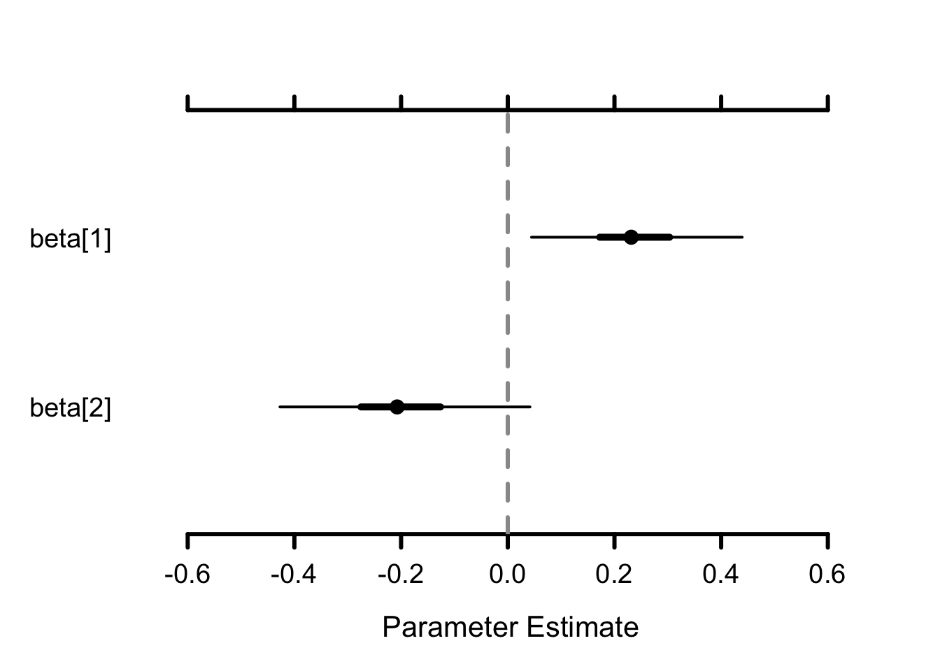
The posterior distribution of the slope (beta[2]) is centered on negative values, suggesting that as water flow increases, survival decreases.
Let’s inspect the time-dependent survival probability:
MCMCplot(object = mcmc.phiflowp, params = "phi", ISB = TRUE)
Survival between 1982 and 1983 (phi[2]) was greatly affected and much lower than on average. This decrease corresponds to the high water flow in 1983 and the flood. These results are in line with our previous findings obtained by considering a discrete covariate for nonflood vs. flood years.
4.8.2 Individual covariates
In the previous section, we learnt how to explain temporal heterogeneity in survival and detection. Heterogeneity could also originate from individual differences between animals. You may think of a diffence in survival between males and females for a discrete covariate example, or size and body mass for examples of a continuous covariate. Let’s illustrate both discrete and continuous covariates on the dipper.
4.8.2.1 Discrete
We first consider a covariate sex that contains 1’s and 2’s indicating the sex of each bird: 1 if male, and 2 if female. We implement the model with sex effect using nested indexing, similarly to the model with flood vs. nonflood years. The section of the NIMBLE code that needs to be amended is:
...
for (i in 1:N){
  gamma[1,1,i] <- phi[sex[i]]      # Pr(alive t -> alive t+1)
  gamma[1,2,i] <- 1 - phi[sex[i]]  # Pr(alive t -> dead t+1)
  gamma[2,1,i] <- 0                # Pr(dead t -> alive t+1)
  gamma[2,2,i] <- 1                # Pr(dead t -> dead t+1)
}
phi[1] ~ dunif(0,1) # male survival
phi[2] ~ dunif(0,1) # female survival
...
After running NIMBLE, we get:
MCMCsummary(object = mcmc.phisexp.ni, round = 2)## mean sd 2.5% 50% 97.5% Rhat n.eff
## p 0.90 0.03 0.84 0.90 0.95 1 643
## phi[1] 0.57 0.03 0.50 0.57 0.64 1 1668
## phi[2] 0.55 0.03 0.48 0.55 0.62 1 1482Male survival (phi[1]) looks very similar to female survival (phi[2]).
4.8.2.2 Continuous
Besides discrete individual covariates, you might want to have continuous individual covariates, e.g. wing length in the dipper example. Note that we’re considering an individual trait that takes the same value whatever the occasion. We consider wing length here, and more precisely its measurement at first detection. We first standardize the covariate:
wing.length.st <- as.vector(scale(dipper$wing_length))
head(wing.length.st)
## [1]  0.7581 -0.8671  0.5260 -1.5637 -1.3315  1.2225
Now we write the model:
hmm.phiwlp <- nimbleCode({
    p ~ dunif(0, 1)             # prior detection
    omega[1,1] <- 1 - p         # Pr(alive t -> non-detected t)
    omega[1,2] <- p             # Pr(alive t -> detected t)
    omega[2,1] <- 1             # Pr(dead t -> non-detected t)
    omega[2,2] <- 0             # Pr(dead t -> detected t)
  for (i in 1:N){
    logit(phi[i]) <- beta[1] + beta[2] * winglength[i]
    gamma[1,1,i] <- phi[i]      # Pr(alive t -> alive t+1)
    gamma[1,2,i] <- 1 - phi[i]  # Pr(alive t -> dead t+1)
    gamma[2,1,i] <- 0           # Pr(dead t -> alive t+1)
    gamma[2,2,i] <- 1           # Pr(dead t -> dead t+1)
  }
  beta[1] ~ dnorm(mean = 0, sd = 1.5)
  beta[2] ~ dnorm(mean = 0, sd = 1.5)
  delta[1] <- 1                 # Pr(alive t = 1) = 1
  delta[2] <- 0                 # Pr(dead t = 1) = 0
  # likelihood
  for (i in 1:N){
    z[i,first[i]] ~ dcat(delta[1:2])
    for (j in (first[i]+1):T){
      z[i,j] ~ dcat(gamma[z[i,j-1], 1:2, i])
      y[i,j] ~ dcat(omega[z[i,j], 1:2])
    }
  }
})
We put the constants in a list:
We write a function for generating initial values:
And we run NIMBLE:
mcmc.phiwlp <- nimbleMCMC(code = hmm.phiwlp,
                          constants = my.constants,
                          data = my.data,
                          inits = initial.values,
                          monitors = parameters.to.save,
                          niter = n.iter,
                          nburnin = n.burnin,
                          nchains = n.chains)
Let’s inspect the numerical summaries for the regression parameters:
MCMCsummary(mcmc.phiwlp, params = "beta", round = 2)## mean sd 2.5% 50% 97.5% Rhat n.eff
## beta[1] 0.25 0.10 0.04 0.25 0.45 1 1472
## beta[2] -0.02 0.09 -0.20 -0.02 0.17 1 1555Wing length does not seem to explain much individual-to-individual variation in survival – the posterior distribution of the slope (beta[2]) is centered on 0 as we can see from the credible interval.
Let’s plot the relationship between survival and wing length. First, we gather the values generated from the posterior distribution of the regression parameters in the two chains:
beta1 <- c(mcmc.phiwlp$chain1[,'beta[1]'], # intercept, chain 1
           mcmc.phiwlp$chain2[,'beta[1]']) # intercept, chain 2
beta2 <- c(mcmc.phiwlp$chain1[,'beta[2]'], # slope, chain 1
           mcmc.phiwlp$chain2[,'beta[2]']) # slope, chain 2
Then we define a grid of values for wing length, and predict survival for each MCMC iteration:
predicted_survival <- matrix(NA,
                             nrow = length(beta1),
                             ncol = length(my.constants$winglength))
for (i in 1:length(beta1)){
  for (j in 1:length(my.constants$winglength)){
    predicted_survival[i,j] <- plogis(beta1[i] +
                               beta2[i] * my.constants$winglength[j])
  }
}
Now we calculate posterior mean and the credible interval (note the ordering):
mean_survival <- apply(predicted_survival, 2, mean)
lci <- apply(predicted_survival, 2, quantile, prob = 2.5/100)
uci <- apply(predicted_survival, 2, quantile, prob = 97.5/100)
ord <- order(my.constants$winglength)
df <- data.frame(wing_length = my.constants$winglength[ord],
                 survival = mean_survival[ord],
                 lci = lci[ord],
                 uci = uci[ord])
Now time to visualize:
df %>%
  ggplot() +
  aes(x = wing_length, y = survival) +
  geom_line() +
  geom_ribbon(aes(ymin = lci, ymax = uci),
              fill = "grey70",
              alpha = 0.5) +
  ylim(0,1) +
  labs(x = "wing length", y = "estimated survival")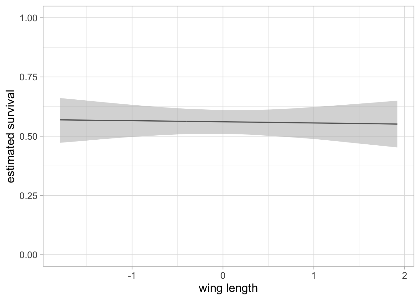
The flat relationship between survival and wing length is confirmed.
4.8.3 Several covariates
You may wish to have an effect of both sex and wing length in a model. Let’s consider an additive effect of both covariates. We use a covariate sex that takes value 0 if male, and 1 if female. We have \(\text{logit}(\phi_i) = \beta_1 + \beta_2 \text{sex}_i + \beta_3 \text{winglength}_i\) for bird \(i\), so that male survival is \(\beta_1 + \beta_3 \text{winglength}_i\) and female survival is \(\beta_1 + \beta_2 + \beta_3 \text{winglength}_i\) (both on the logit scale). The relationship between survival and wing length is parallel between males and females, on the logit scale, and the gap between the two is measured by \(\beta_2\) (hence the term additive effect).
The NIMBLE code is:
hmm.phisexwlp <- nimbleCode({
  p ~ dunif(0, 1)               # prior detection
  omega[1,1] <- 1 - p           # Pr(alive t -> non-detected t)
  omega[1,2] <- p               # Pr(alive t -> detected t)
  omega[2,1] <- 1               # Pr(dead t -> non-detected t)
  omega[2,2] <- 0               # Pr(dead t -> detected t)
  for (i in 1:N){
    logit(phi[i])<-beta[1]+beta[2]*sex[i]+beta[3]*winglength[i]
    gamma[1,1,i] <- phi[i]      # Pr(alive t -> alive t+1)
    gamma[1,2,i] <- 1 - phi[i]  # Pr(alive t -> dead t+1)
    gamma[2,1,i] <- 0           # Pr(dead t -> alive t+1)
    gamma[2,2,i] <- 1           # Pr(dead t -> dead t+1)
  }
  beta[1] ~ dnorm(mean = 0, sd = 1.5) # intercept male
  beta[2] ~ dnorm(mean = 0, sd = 1.5) # diff bw male and female
  beta[3] ~ dnorm(mean = 0, sd = 1.5) # slope wing length
  delta[1] <- 1                 # Pr(alive t = 1) = 1
  delta[2] <- 0                 # Pr(dead t = 1) = 0
  # likelihood
  for (i in 1:N){
    z[i,first[i]] ~ dcat(delta[1:2])
    for (j in (first[i]+1):T){
      z[i,j] ~ dcat(gamma[z[i,j-1], 1:2, i])
      y[i,j] ~ dcat(omega[z[i,j], 1:2])
    }
  }
})
We put constants and data in lists:
first <- apply(y, 1, function(x) min(which(x !=0)))
wing.length.st <- as.vector(scale(dipper$wing_length))
my.constants <- list(N = nrow(y),
                     T = ncol(y),
                     first = first,
                     winglength = wing.length.st,
                     sex = if_else(dipper$sex == "M", 0, 1))
my.data <- list(y = y + 1)
We write a fuction to generate initial values:
zinits <- y
zinits[zinits == 0] <- 1
initial.values <- function() list(beta = rnorm(3,0,2),
                                  p = runif(1,0,1),
                                  z = zinits)
We specify the parameters to be monitored:
parameters.to.save <- c("beta", "p")The MCMC details (note that we need to increase the number of iterations to achieve satisfying effective sample sizes):
n.iter <- 5000*4
n.burnin <- 1000
n.chains <- 2
And now we run NIMBLE:
mcmc.phisexwlp <- nimbleMCMC(code = hmm.phisexwlp,
                             constants = my.constants,
                             data = my.data,
                             inits = initial.values,
                             monitors = parameters.to.save,
                             niter = n.iter,
                             nburnin = n.burnin,
                             nchains = n.chains)
Let’s display numerical summaries for all parameters:
MCMCsummary(mcmc.phisexwlp, round = 2)## mean sd 2.5% 50% 97.5% Rhat n.eff
## beta[1] 0.52 0.24 0.05 0.52 0.99 1 466
## beta[2] -0.53 0.43 -1.37 -0.53 0.30 1 447
## beta[3] -0.25 0.21 -0.65 -0.25 0.16 1 530
## p 0.90 0.03 0.83 0.90 0.95 1 3141The slope beta[3] is the same for both males and females. Although its posterior mean is negative, its crebible interval suggests that its posterior distribution largely encompasses 0, therefore a very weak signal, if any.
Let’s visualize survival as a function of wing length for both sexes. First we put together the values from the two chains we generated in the posterior distributions of the regression parameters:
beta1 <- c(mcmc.phisexwlp$chain1[,'beta[1]'], # beta1 chain 1
           mcmc.phisexwlp$chain2[,'beta[1]']) # beta1 chain 2
beta2 <- c(mcmc.phisexwlp$chain1[,'beta[2]'], # beta2 chain 1
           mcmc.phisexwlp$chain2[,'beta[2]']) # beta2 chain 2
beta3 <- c(mcmc.phisexwlp$chain1[,'beta[3]'], # beta3 chain 1
           mcmc.phisexwlp$chain2[,'beta[3]']) # beta3 chain 2
We get survival estimates for each MCMC iteration:
predicted_survivalM <- matrix(NA, nrow = length(beta1),
                              ncol=length(my.constants$winglength))
predicted_survivalF <- matrix(NA, nrow = length(beta1),
                              ncol=length(my.constants$winglength))
for (i in 1:length(beta1)){
  for (j in 1:length(my.constants$winglength)){
    predicted_survivalM[i,j] <- plogis(beta1[i] +
                                beta3[i]*my.constants$winglength[j])
    predicted_survivalF[i,j] <- plogis(beta1[i] +
                                beta2[i] +
                                beta3[i]*my.constants$winglength[j])
  }
}
From here, we may calculate posterior mean and credible intervals:
mean_survivalM <- apply(predicted_survivalM, 2, mean)
lciM <- apply(predicted_survivalM, 2, quantile, prob = 2.5/100)
uciM <- apply(predicted_survivalM, 2, quantile, prob = 97.5/100)
mean_survivalF <- apply(predicted_survivalF, 2, mean)
lciF <- apply(predicted_survivalF, 2, quantile, prob = 2.5/100)
uciF <- apply(predicted_survivalF, 2, quantile, prob = 97.5/100)
ord <- order(my.constants$winglength)
df <- data.frame(wing_length = c(my.constants$winglength[ord],
                                 my.constants$winglength[ord]),
                 survival = c(mean_survivalM[ord],
                              mean_survivalF[ord]),
                 lci = c(lciM[ord],lciF[ord]),
                 uci = c(uciM[ord],uciF[ord]),
                 sex = c(rep("male", length(mean_survivalM)),
                         rep("female", length(mean_survivalF))))
Now on a plot:
if (params$bw) {
  df %>%
    ggplot(aes(x = wing_length, y = survival, color = sex, fill = sex)) +
    geom_line() +
    geom_ribbon(aes(ymin = lci, ymax = uci), alpha = 0.3) +
    ylim(0, 1) +
    labs(x = "wing length",
         y = "estimated survival",
         color = "", fill = "") +
    scale_color_manual(values = c("black", "grey40")) +
    scale_fill_manual(values  = c("grey70", "grey10"))
} else {
  df %>%
    ggplot() +
    aes(x = wing_length, y = survival, color = sex) +
    geom_line() +
    geom_ribbon(aes(ymin = lci, ymax = uci, fill = sex), alpha = 0.5) +
    ylim(0,1) +
    labs(x = "wing length",
         y = "estimated survival",
         color = "", fill = "")
}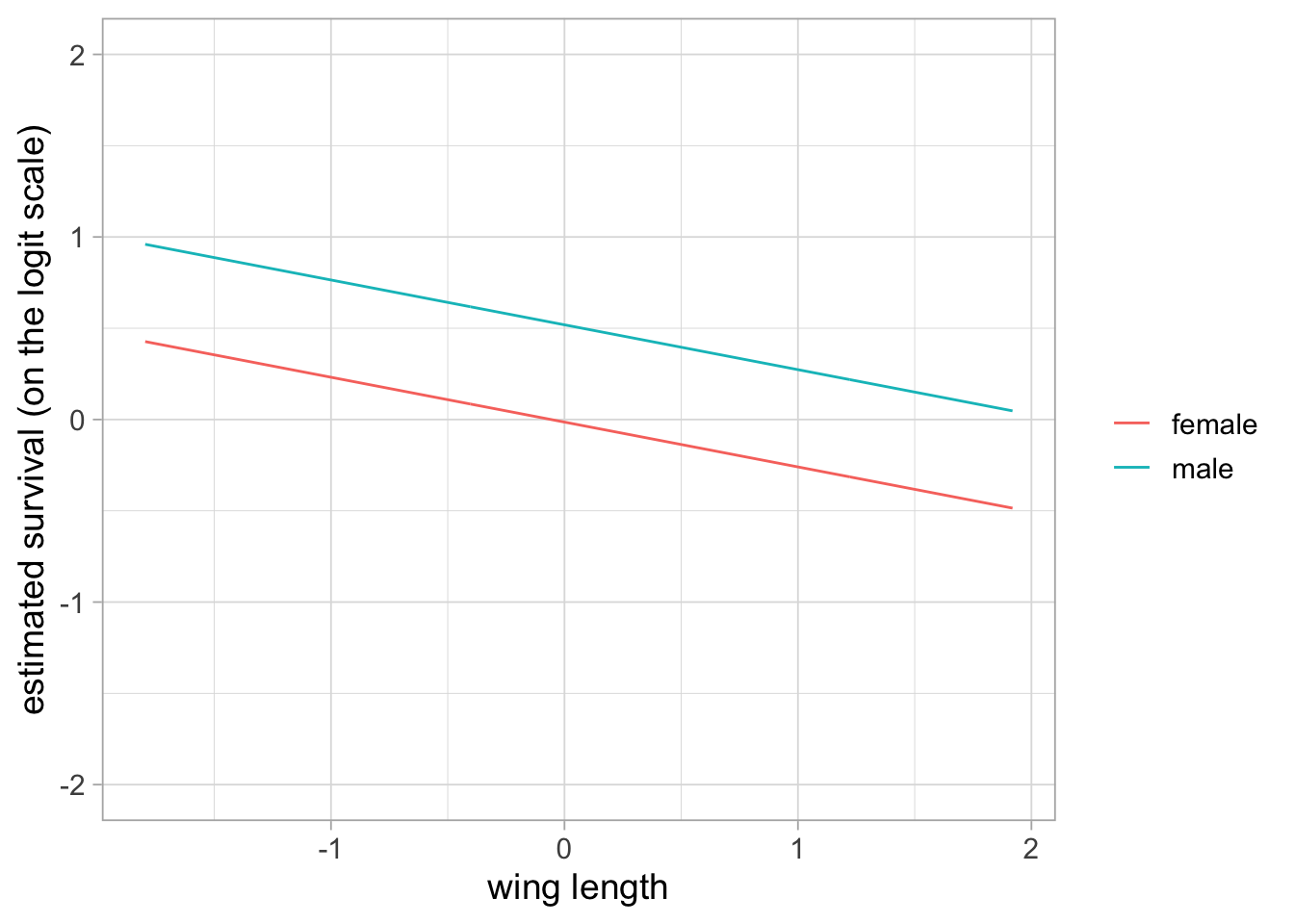
Note that the two curves are not exactly parallel because we back-transformed the linear part of the relationship between survival and wing length. You may check that parallelism occurs on the logit scale:
predicted_lsurvivalM <- matrix(NA, nrow = length(beta1),
                              ncol = length(my.constants$winglength))
predicted_lsurvivalF <- matrix(NA, nrow = length(beta1),
                              ncol = length(my.constants$winglength))
for (i in 1:length(beta1)){
  for (j in 1:length(my.constants$winglength)){
    predicted_lsurvivalM[i,j] <- beta1[i] +
      beta3[i] * my.constants$winglength[j]
    predicted_lsurvivalF[i,j] <- beta1[i] + beta2[i] +
      beta3[i] * my.constants$winglength[j]
  }
}
mean_lsurvivalM <- apply(predicted_lsurvivalM, 2, mean)
mean_lsurvivalF <- apply(predicted_lsurvivalF, 2, mean)
ord <- order(my.constants$winglength)
df <- data.frame(wing_length = c(my.constants$winglength[ord],
                                 my.constants$winglength[ord]),
                 survival = c(mean_lsurvivalM[ord],
                              mean_lsurvivalF[ord]),
                 sex = c(rep("male", length(mean_lsurvivalM)),
                         rep("female", length(mean_lsurvivalF))))

if (params$bw) {
  df %>%
    ggplot(aes(x = wing_length, y = survival, color = sex, linetype = sex)) +
    geom_line(linewidth = 1) +
    ylim(-2, 2) +
    labs(x = "wing length",
         y = "estimated survival (on the logit scale)",
         color = "", linetype = "") +
    scale_color_manual(values = c("black", "grey70")) +
    scale_linetype_manual(values = c("solid", "solid"))
} else {
  df %>%
    ggplot() +
    aes(x = wing_length, y = survival, color = sex) +
    geom_line() +
    ylim(-2,2) +
    labs(x = "wing length",
         y = "estimated survival (on the logit scale)",
         color = "")
}
4.8.4 Random effects
If individual variation in survival is not fully explained by our covariates, we may add random effects through \(\text{logit}(\phi_i) = \beta_1 + \beta_2 x_i + \varepsilon_i\) where \(\varepsilon_i \sim N(0,\sigma^2)\). We consider individual variation in this section, but the reasoning holds for temporal variation. In essence, we are treating the individual survival probabilities \(\phi_i\) as a sample from a population of survival probabilities, and we assume a normal distribution with mean the linear component (with or without a covariate) and standard deviation \(\sigma\). The variation that is unexplained by the covariate \(x_i\) is measured by the variation \(\sigma\) in the residuals \(\varepsilon_i\).
Why is it important? Ignoring individual heterogeneity generated by individuals having contrasted performances over life may mask senescence or hamper the understanding of life history trade-offs. Overall, failing to incorporate unexplained residual variance may induce bias in parameter estimates and lead to detecting an effect of the covariate more often than it should be.
Let’s go back to our dipper example with wing length as a covariate, and write the NIMBLE code:
hmm.phiwlrep <- nimbleCode({
    p ~ dunif(0, 1)             # prior detection
    omega[1,1] <- 1 - p         # Pr(alive t -> non-detected t)
    omega[1,2] <- p             # Pr(alive t -> detected t)
    omega[2,1] <- 1             # Pr(dead t -> non-detected t)
    omega[2,2] <- 0             # Pr(dead t -> detected t)
  for (i in 1:N){
    logit(phi[i]) <- beta[1] + beta[2] * winglength[i] + eps[i]
    eps[i] ~ dnorm(mean = 0, sd = sdeps)
    gamma[1,1,i] <- phi[i]      # Pr(alive t -> alive t+1)
    gamma[1,2,i] <- 1 - phi[i]  # Pr(alive t -> dead t+1)
    gamma[2,1,i] <- 0           # Pr(dead t -> alive t+1)
    gamma[2,2,i] <- 1           # Pr(dead t -> dead t+1)
  }
  beta[1] ~ dnorm(mean = 0, sd = 1.5)
  beta[2] ~ dnorm(mean = 0, sd = 1.5)
  sdeps ~ dunif(0, 10)
  delta[1] <- 1                 # Pr(alive t = 1) = 1
  delta[2] <- 0                 # Pr(dead t = 1) = 0
  # likelihood
  for (i in 1:N){
    z[i,first[i]] ~ dcat(delta[1:2])
    for (j in (first[i]+1):T){
      z[i,j] ~ dcat(gamma[z[i,j-1], 1:2, i])
      y[i,j] ~ dcat(omega[z[i,j], 1:2])
    }
  }
})
The prior on the standard deviation of the random effect is uniform between 0 and 10.
We now write a function for generating initial values:
initial.values <- function() list(beta = rnorm(2,0,1.5),
                                  sdeps = runif(1,0,3),
                                  p = runif(1,0,1),
                                  z = zinits)
We specify the parameters to be monitored:
parameters.to.save <- c("beta", "sdeps", "p")We increase the number of iterations and the length of the burn-in period to reach better convergence:
n.iter <- 10000
n.burnin <- 5000
n.chains <- 2
And finally, we run NIMBLE:
mcmc.phiwlrep <- nimbleMCMC(code = hmm.phiwlrep,
                            constants = my.constants,
                            data = my.data,
                            inits = initial.values,
                            monitors = parameters.to.save,
                            niter = n.iter,
                            nburnin = n.burnin,
                            nchains = n.chains)
We inspect the numerical summaries:
MCMCsummary(mcmc.phiwlrep, round = 2)## mean sd 2.5% 50% 97.5% Rhat n.eff
## beta[1] 0.22 0.12 -0.02 0.22 0.44 1.24 1335
## beta[2] -0.01 0.10 -0.20 -0.01 0.19 1.02 1894
## p 0.90 0.03 0.84 0.90 0.95 1.03 752
## sdeps 0.27 0.25 0.01 0.16 0.83 4.68 12The effective sample size for the standard deviation of the random effect is very low. Let’s try something else, which means that the MCMC chains are exploring that parameter space inefficiently. A common strategy to address this problem is to reparameterize the model using a non-centered formulation.
In the centered parameterization we’ve used so far, the random effect is expressed directly in terms of its variance (or standard deviation). This often creates strong correlations between the random effects and their variance parameter, which in turn can slow down mixing and reduce the effective sample size. In the non-centered parameterization, we instead separate the structure of the random effect from its scale. In practice, we introduce a standardized random effect \(\varepsilon_i \sim N(0,1)\) and then multiply it by the standard deviation \(\sigma\). This decouples the randomness from the scale parameter and usually improves sampling efficiency. In code, this looks like:
...
  for (i in 1:N){
    logit(phi[i])<-beta[1]+beta[2]*winglength[i] + sdeps * eps[i]
    eps[i] ~ dnorm(mean = 0, sd = 1)
...
After running NIMBLE, we inspect the numerical summaries, and see that effective sample sizes are much better:
MCMCsummary(mcmc.phiwlrep, round = 2)## mean sd 2.5% 50% 97.5% Rhat n.eff
## beta[1] 0.21 0.12 -0.04 0.21 0.43 1.00 1202
## beta[2] -0.01 0.10 -0.20 -0.01 0.19 1.00 1789
## p 0.90 0.03 0.83 0.90 0.95 1.01 790
## sdeps 0.40 0.26 0.02 0.37 0.95 1.01 1704.8.5 Individual time-varying covariates
So far, we allowed covariates to vary along a single dimension, either time or individual. What if we need to consider a covariate that varies from one animal to the other, and over time. Think of age for example, its value is specific to each individual, and it (sadly) changes over time.
Age has a particular meaning in the capture-recapture framework. It is the time elapsed since first encounter, which is a proxy of true age, but not true age. If age is known at first encounter, then it is true age. For example, if the dippers were marked as young, then we would have the true biological age of each bird.
The convenient thing is that age has no missing value because age at \(t+1\) is just age at \(t\) to which we add 1. This suggests a way to code the age effect in NIMBLE as follows:
hmm.phiage.in <- nimbleCode({
  p ~ dunif(0, 1)                     # prior detection
  omega[1,1] <- 1 - p                 # Pr(alive t -> non-detected t)
  omega[1,2] <- p                     # Pr(alive t -> detected t)
  omega[2,1] <- 1                     # Pr(dead t -> non-detected t)
  omega[2,2] <- 0                     # Pr(dead t -> detected t)
  for (i in 1:N){
    for (t in first[i]:(T-1)){
    # phi1 = beta1 + beta2; phi1+ = beta1
    logit(phi[i,t]) <- beta[1] + beta[2] * equals(t, first[i])
    gamma[1,1,i,t] <- phi[i,t]        # Pr(alive t -> alive t+1)
    gamma[1,2,i,t] <- 1 - phi[i,t]    # Pr(alive t -> dead t+1)
    gamma[2,1,i,t] <- 0               # Pr(dead t -> alive t+1)
    gamma[2,2,i,t] <- 1               # Pr(dead t -> dead t+1)
    }
  }
  beta[1] ~ dnorm(mean = 0, sd = 1.5) # phi1+
  beta[2] ~ dnorm(mean = 0, sd = 1.5) # phi1 - phi1+
  phi1plus <- plogis(beta[1])         # phi1+
  phi1 <- plogis(beta[1] + beta[2])   # phi1
  delta[1] <- 1                       # Pr(alive t = 1) = 1
  delta[2] <- 0                       # Pr(dead t = 1) = 0
  # likelihood
  for (i in 1:N){
    z[i,first[i]] ~ dcat(delta[1:2])
    for (j in (first[i]+1):T){
      z[i,j] ~ dcat(gamma[z[i,j-1], 1:2, i, j-1])
      y[i,j] ~ dcat(omega[z[i,j], 1:2])
    }
  }
})
Here we used equals(t, first[i]) which renders 1 when \(t\) is the first encounter first[i] and 0 otherwise. Therefore we distinguish survival over the first interval after first encounter \(\phi_1\) (logit(phi[i,t]) <- beta[1] + beta[2]) from survival afterwards \(\phi_{1+}\) (logit(phi[i,t]) <- beta[1]).
We put all constants in a list:
first <- apply(y, 1, function(x) min(which(x !=0)))
my.constants <- list(N = nrow(y),
                     T = ncol(y),
                     first = first)
And the data in a list:
my.data <- list(y = y + 1)We write a function to generate initial values:
zinits <- y
zinits[zinits == 0] <- 1
initial.values <- function() list(beta = rnorm(2,0,5),
                                  p = runif(1,0,1),
                                  z = zinits)
And specify the parameters to be monitored:
parameters.to.save <- c("phi1", "phi1plus", "p")We now run NIMBLE:
mcmc.phi.age.in <- nimbleMCMC(code = hmm.phiage.in,
                              constants = my.constants,
                              data = my.data,
                              inits = initial.values,
                              monitors = parameters.to.save,
                              niter = n.iter,
                              nburnin = n.burnin,
                              nchains = n.chains)
We display the results:
MCMCsummary(mcmc.phi.age.in, round = 2)## mean sd 2.5% 50% 97.5% Rhat n.eff
## p 0.90 0.03 0.83 0.90 0.95 1.00 738
## phi1 0.56 0.03 0.49 0.56 0.62 1.00 1624
## phi1plus 0.57 0.04 0.49 0.57 0.64 1.01 506Age or time elapsed since first encounter does not seem to have an effect on survival here.
Another method to include an age effect is to create an individual by time covariate and use nested indexing (as in the flood/nonflood example) to distinguish survival over the interval after first detection from survival afterwards:
age <- matrix(NA, nrow = nrow(y), ncol = ncol(y) - 1)
for (i in 1:nrow(age)){
  for (j in 1:ncol(age)){
    if (j == first[i]) age[i,j] <- 1 # age = 1
    if (j > first[i]) age[i,j] <- 2  # age > 1
  }
}
Now we may write the NIMBLE code for this model. We just need to remember that survival is no longer defined on the logit scale as in the previous model, so we simply use uniform priors:
hmm.phiage.out <- nimbleCode({
  p ~ dunif(0, 1)                   # prior detection
  omega[1,1] <- 1 - p               # Pr(alive t -> non-detected t)
  omega[1,2] <- p                   # Pr(alive t -> detected t)
  omega[2,1] <- 1                   # Pr(dead t -> non-detected t)
  omega[2,2] <- 0                   # Pr(dead t -> detected t)
  for (i in 1:N){
    for (t in first[i]:(T-1)){
    phi[i,t] <- beta[age[i,t]]      # beta1 = phi1, beta2 = phi1+
    gamma[1,1,i,t] <- phi[i,t]      # Pr(alive t -> alive t+1)
    gamma[1,2,i,t] <- 1 - phi[i,t]  # Pr(alive t -> dead t+1)
    gamma[2,1,i,t] <- 0             # Pr(dead t -> alive t+1)
    gamma[2,2,i,t] <- 1             # Pr(dead t -> dead t+1)
    }
  }
  beta[1] ~ dunif(0, 1) # phi1
  beta[2] ~ dunif(0, 1) # phi1+
  phi1 <- beta[1]
  phi1plus <- beta[2]
  delta[1] <- 1                     # Pr(alive t = 1) = 1
  delta[2] <- 0                     # Pr(dead t = 1) = 0
  # likelihood
  for (i in 1:N){
    z[i,first[i]] ~ dcat(delta[1:2])
    for (j in (first[i]+1):T){
      z[i,j] ~ dcat(gamma[z[i,j-1], 1:2, i, j-1])
      y[i,j] ~ dcat(omega[z[i,j], 1:2])
    }
  }
})
We put all constants in a list, including the age covariate:
first <- apply(y, 1, function(x) min(which(x !=0)))
my.constants <- list(N = nrow(y),
                     T = ncol(y),
                     first = first,
                     age = age)
We re-write a function to generate initial values:
zinits <- y
zinits[zinits == 0] <- 1
initial.values <- function() list(beta = runif(2,0,1),
                                  p = runif(1,0,1),
                                  z = zinits)
And we run NIMBLE:
mcmc.phi.age.out <- nimbleMCMC(code = hmm.phiage.out,
                               constants = my.constants,
                               data = my.data,
                               inits = initial.values,
                               monitors = parameters.to.save,
                               niter = n.iter,
                               nburnin = n.burnin,
                               nchains = n.chains)
We display numerical summaries for the model parameters, and acknowledge that we obtain similar results to the other parameterization:
MCMCsummary(mcmc.phi.age.out, round = 2)## mean sd 2.5% 50% 97.5% Rhat n.eff
## p 0.90 0.03 0.84 0.90 0.95 1.01 793
## phi1 0.55 0.03 0.48 0.55 0.62 1.01 1736
## phi1plus 0.57 0.04 0.50 0.57 0.64 1.00 2064Like I mentioned earlier, age is easy to deal with as it does not contain missing values. Now think of size or body mass for a minute. The problem is that we cannot record size or body mass when an animal is non-detected. The easiest way to cope with individual time-varying covariates is to discretize e.g. in small, medium and large as in Chapter 5. Another option is to come up with a model for the covariate and fill in missing values by simulating from this model.
4.9 Why Bayes? Incorporate prior information
4.9.1 Prior elicitation
Before we close this section, I’d like to cover one last topic. Think again of the CJS model with constant parameters. So far, we have assumed a non-informative prior on survival \(\text{Beta}(1,1) = \text{Uniform}(0,1)\). With this prior, we have seen in Section 4.5 that mean posterior survival is \(\phi = 0.56\) with credible interval \([0.52,0.62]\).
The thing is that we know a lot about passerines and it is a shame not to be able to use this information and act as if we have to start from scratch and know nothing.
We illustrate how to incorporate prior information by acknowledging that species with similar body masses have similar survival. By gathering information on several other European passerines than the dipper, let’s assume we have built a regression of survival vs. body mass – an allometric relationship.
Now knowing dippers weigh on average 59.8g, we’re in the position to build a prior for dipper survival probability by predicting its value using the regression. We obtain a predicted survival of 0.57 and a standard deviation of 0.075. Using an informative prior phi ~ dnorm(0.57, sd = 0.073) in NIMBLE instead of our phi ~ dunif(0,1), we get a mean posterior of \(0.56\) with credible interval \([0.52, 0.61]\). There’s barely no difference with the non-informative prior, quite a disappointment.
Now let’s assume that we had only the three first years of data, what would have happened? We fit the model with constant parameters with both the non-informative and informative priors to the dataset from which we delete the final 4 years of data. Now the benefit of using the prior information becomes clear as the credible interval when prior information is ignored has a width of 0.53, which is more than twice as much as when prior information is used (0.24), illustrating the increased precision provided by the prior. We may assess visually this gain in precision by comparing the survival posterior distributions with and without informative prior:
If the aim is to get an estimate of survival, Gilbert did not have to conduct further data collection after 3 years, and he could have reached the same precision as with 7 years of data by using prior information derived from body mass. In brief, the prior information was worth 4 years of field data. Of course, this is assuming that the ecological question remains the same whether you have 3 or 7 years of data, which is unlikely to be the case, as with long-term data, there is so much we can ask, more than “just” what annual survival probability is.
4.9.2 Moment matching
The prior phi ~ dnorm(0.57, sd = 0.073) is not entirely satisfying because it is not constrained to be positive or less than one, which is the minimum for a probability (of survival) to be well defined. In our specific example, the prior distribution is centered on positive values far from 0, and the standard deviation is small enough so that the chances to get values smaller than 0 or higher than 1 are null (to convince yourself, just type in hist(rnorm(1000, mean = 0.57, sd = 0.073)) in R). Can we do better? The answer is yes.
Remember the Beta distribution? Recall that the Beta distribution is a continuous distribution with values between 0 and 1, which is very convenient to specify priors for survival and detection probabilities. Besides we know everything about the Beta distribution, in particular its mean and variance. If \(X \sim Beta(\alpha,\beta)\), then the mean and (variance) of \(X\) are \(\mu = \text{E}(X) = \frac{\alpha}{\alpha + \beta}\) and \(\sigma^2 = \text{Var}(X) = \frac{\alpha\beta}{(\alpha + \beta)^2 (\alpha + \beta + 1)}\).
In the capture-recapture example, we know a priori that the mean of the probability we’re interested in is \(\mu = 0.57\) and its variance is \(\sigma^2 = 0.073^2\). Parameters \(\mu\) and \(\sigma^2\) are seen as the moments of a \(Beta(\alpha,\beta)\) distribution. Now we look for values of \(\alpha\) and \(\beta\) that match the observed moments of the Beta distribution \(\mu\) and \(\sigma^2\). We need another set of equations:
\[\alpha = \bigg(\frac{1-\mu}{\sigma^2}- \frac{1}{\mu} \bigg)\mu^2\] \[\beta = \alpha \bigg(\frac{1}{\mu}-1\bigg)\] For our model, that means:
(alpha <- ( (1 - 0.57)/(0.073*0.073) - (1/0.57) )*0.57^2)
## [1] 25.65
(beta <- alpha * ( (1/0.57) - 1))
## [1] 19.35
Now we simply have to use phi ~ dbeta(25.6,19.3) as a prior instead of our phi ~ dnorm(0.57, sd = 0.073).
4.10 Summary
The CJS model is a HMM with time-varying parameters to account for variation due to environmental conditions in survival or to sampling effort in detection.
Covariates can be considered to try and explain temporal and/or individual variation in survival and detection probabilities. If needed, random effects can be added to cope with unexplained variation.
For model comparison, the WAIC can be used to evaluate the relative predictive performance of capture-recapture models.
Statistical models rely on assumptions, and the CJS model makes no exception. There are procedures to assess the goodness of fit of the CJS model to capture-recapture data.
4.11 Suggested reading
Buckland (2016) provides a historical perspective on the CJS model and anecdotes. The monography by Lebreton et al. (1992) is a must-read to better understand the CJS model and its applications. The HMM formulation of the CJS model was proposed by Gimenez et al. (2007) and Royle (2008).
Gimenez, Morgan, and Brooks (2009) deals with parameter redundancy in capture-recapture models in a Bayesian framework. For an exhaustive treatment, see Cole (2020) excellent book.
Relative to model comparison, I warmly recommend McElreath (2020) to better understand WAIC, with the accompanying video, see https://www.youtube.com/watch?v=vSjL2Zc-gEQ. The paper by Gelman, Hwang, and Vehtari (2014) is also much helpful.
On posterior predictive checks, you may check out Conn et al. (2018). The
R2ucarepackage is introduced by Gimenez et al. (2018).Temporal heterogeneity is addressed in papers by Grosbois et al. (2008) and Frederiksen et al. (2014), while individual heterogeneity is reviewed by Gimenez, Cam, and Gaillard (2018).
Regarding covariates, I did not use the formalization of linear models and sticked to an intuitive (hopefully) illustration of the use of covariates. More details can be found in Chapter 6 of Cooch and White (2017).
The example on how to incorporate prior information is from McCarthy and Masters (2005).