5 Sites and states

5.1 Introduction

In this fifth chapter, you will learn about the Arnason-Schwarz model that allows estimating transitions between sites and states based on capture-recapture data. You will also see how to deal with uncertainty in the assignment of states to individuals.

5.2 The Arnason-Schwarz (AS) model

In Chapter 4, we got acquainted with the Cormack-Jolly-Seber (CJS) model which accommodates transitions between the states alive and dead while accounting for imperfect detection. It is often the case that besides being alive, more detailed information is collected on the state of animals when they are detected. For example, if the study area is split into several discrete sites, you may record where an animal is detected, the state being now alive in this particular site. The Arnason-Schwarz (AS) model can be viewed as an extension to the CJS model in which we estimate movements between sites on top of survival. The AS model is named after the two statisticians – Neil Arnason and Carl Schwarz – who came up with the idea.

5.2.1 Theory

Let’s assume for now that we have two sites, say 1 and 2. The way we usually think of analyzing the data is to start from the detections and non-detections and infer the transitions between sites and movements. Schematically, when a animal is detected in site 1 or site 2, it obviously means that it is alive in that site, whereas when it is not detected, it may be dead or alive in either site. Schematically, we have:

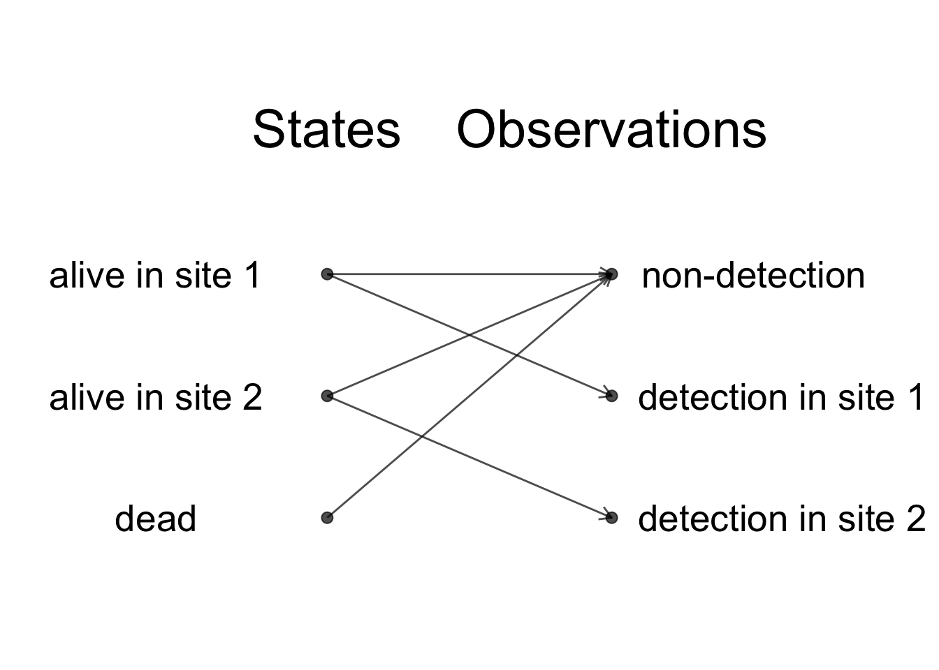
Observations and states are indeed closely related, but we do not have a perfect states to observations correspondence, and the HMM framework will help you make the distinction clear, which in turn will make the modelling easier. Usually, we focus our energy on the observations but what we’d really like is to spend time thinking of the ecological processes that we observed imperfectly. In the HMM framework, when we are to build a model, we think of the states and their dynamic over time, and these states emit the observations we’re given to make. Going back to the our example, when an animal is alive in either site, it may get detected in that site or go undetected. When an animal is dead, then it goes undetected for sure. Schematically, we obtain:

We have $z = 1$ for alive in site 1, $z = 2$ for alive in site 2 and $z = 3$ for dead. We will code $y = 1$ for non-detected, $y = 2$ for detected in site 1 and $y = 3$ for detected in site 2. The parameters are:
- $\pi^r$ is the probability the a newly encountered individual is in state $r$;
- $p_t^r$ is the probability of detection at $t$ for a bird in site $r$ at $t$;
- $\phi_t^r$ is the survival probability for birds in site $r$ at between $t$ and $t+1$;
- $\psi_t^{rs}$ is the probability of being in site $s$ at time $t+1$ for animals that were in site $r$ at $t$ and have survived to $t+1$, in short movement conditional on survival.

These parameters can be modelled as functions of covariates as in Section 4.8. But for now we will drop the time index for simplicity.

We follow the presentation of HMM as in Chapter 3. Let’s start with the vector of initial states. At first encounter, an animal may be alive in site 1 with probability $\pi^1$ or in site 2 with the complementary probability $1 - \pi^{1}$, but it cannot be dead. Therefore, we have:

\[\begin{matrix} & \\ \mathbf{\delta} = \left ( \vphantom{ \begin{matrix} 12 \end{matrix} } \right . \end{matrix} \hspace{-1.2em} \begin{matrix} z_t=1 & z_t=2 & z_t=3 \\ \hdashline \pi^1 & 1 - \pi^{1} & 0\\ \end{matrix} \hspace{-0.2em} \begin{matrix} & \\ \left . \vphantom{ \begin{matrix} 12 \end{matrix} } \right ) \begin{matrix} \end{matrix} \end{matrix}\]

We move on to the transition matrix which connects the states at $t-1$ in rows to the states at $t$ in columns. For example, the probability of moving from site 1 at $t-1$ to site $2$ at $t$ is the product of the survival probability in site 1 over that time interval, times the probability of moving from site 1 to 2 for those animals who survived. We have:

\[\begin{matrix} & \\ \mathbf{\Gamma} = \left ( \vphantom{ \begin{matrix} 12 \\ 12 \\ 12 \end{matrix} } \right . \end{matrix} \hspace{-1.2em} \begin{matrix} z_{t}=1 & z_{t}=2 & z_{t}=3 \\ \hdashline \phi^1 (1-\psi^{12}) & \phi^1 \psi^{12} & 1 - \phi^1\\ \phi^2 \psi^{21} & \phi^2 (1-\psi^{21}) & 1 - \phi^2\\ 0 & 0 & 1 \end{matrix} \hspace{-0.2em} \begin{matrix} & \\ \left . \vphantom{ \begin{matrix} 12 \\ 12 \\ 12 \end{matrix} } \right ) \begin{matrix} z_{t-1}=1 \\ z_{t-1}=2 \\ z_{t-1}=3 \end{matrix} \end{matrix}\]

Finally, the observation matrix relates the states an animal is in at $t$ in rows to the observations at $t$ in columns. If an animal is dead ($z_t=3$), it cannot be detected ($\Pr(y_t=1|z_t=3)=\Pr(y_t=2|z_t=3)=0$ and $\Pr(y_t=3|z_t=3)=1$), whereas when it is alive in either site, it can be detected or not. We have:

\[\begin{matrix} & \\ \mathbf{\Omega} = \left ( \vphantom{ \begin{matrix} 12 \\ 12 \\ 12 \end{matrix} } \right . \end{matrix} \hspace{-1.2em} \begin{matrix} y_t=1 & y_t=2 & y_t=3 \\ \hdashline 1 - p^1 & p^1 & 0\\ 1 - p^2 & 0 & p^2\\ 1 & 0 & 0 \end{matrix} \hspace{-0.2em} \begin{matrix} & \\ \left . \vphantom{ \begin{matrix} 12 \\ 12 \\ 12 \end{matrix} } \right ) \begin{matrix} z_{t}=1 \\ z_{t}=2 \\ z_{t}=3 \end{matrix} \end{matrix}\]

The vector of initial state probabilities sums up to one, as well as the rows of the transition and observation matrices.

5.3 Fitting the AS model

5.3.1 Geese data

To introduce this chapter, we will use data on the Canada goose (Branta canadensis; geese hereafter) kindly provided by Jay Hestbeck (Figure 4.2).

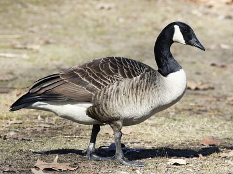
Figure 5.1: Canada goose (Branta canadensis). Credit: Max McCarthy.

In total, 21277 geese were captured, marked with coded neck bands and recaptured between 1984 and 1989 in their wintering locations. Specifically, geese were monitored in the Atlantic flyway, in large areas along the East coast of the USA, namely 3 sites in the mid–Atlantic (New York, Pennsylvania, New Jersey), Chesapeake (Delaware, Maryland, Virginia), and Carolinas (North and South Carolina). Birds were adults and sub-adults when banded.

You may see the data below:

y <- read_csv("dat/geese.csv") %>% as.matrix()
head(y)
##      year_1984 year_1985 year_1986 year_1987 year_1988
## [1,]         0         2         2         0         0
## [2,]         0         0         0         0         0
## [3,]         0         0         0         1         0
## [4,]         0         0         2         0         0
## [5,]         0         3         0         0         3
## [6,]         0         0         0         2         0
##      year_1989
## [1,]         0
## [2,]         2
## [3,]         0
## [4,]         0
## [5,]         2
## [6,]         0

The six columns are years in which the geese were captured, banded and recapture. A 0 stands for a non-detection, and detections were coded in the 3 wintering sites 1, 2 and 3 for mid–Atlantic, Chesapeake and Carolinas respectively. This is only a subsample of 500 individuals of the whole dataset that I will use for illustration here.

5.3.2 NIMBLE implementation

To write the NIMBLE code corresponding to the AS model, we will make our life easier and start with 2 sites only – we drop the Carolinas wintering site for now. We replace all 3’s by 0’s in the dataset:

y[y==3] <- 0

Also we consider parameters constant over time.

We start with comments to define the quantities – parameters, states and observations – we will use in the NIMBLE code:

multisite <- nimbleCode({
  # -------------------------------------------------
  # Parameters:
  # phi1: survival probability site 1
  # phi2: survival probability site 2
  # psi12: movement probability from site 1 to site 2
  # psi21: movement probability from site 2 to site 1
  # p1: detection probability site 1
  # p2: detection probability site 2
  # -------------------------------------------------
  # States (z):
  # 1 alive at site 1
  # 2 alive at site 2
  # 3 dead
  # Observations (y):
  # 1 not seen
  # 2 seen at site 1
  # 3 seen at site 2
  # -------------------------------------------------
...

The we specify priors for the survival, transition and detection probabilities:

multisite <- nimbleCode({
...
  # Priors
  phi1 ~ dunif(0, 1)
  phi2 ~ dunif(0, 1)
  psi12 ~ dunif(0, 1)
  psi21 ~ dunif(0, 1)
  p1 ~ dunif(0, 1)
  p2 ~ dunif(0, 1)
...

We now write the vector of initial state probabilities:

multisite <- nimbleCode({
...
  # initial state probabilities
  delta[1] <- pi1          # Pr(alive in 1 at t = first)
  delta[2] <- 1 - pi1      # Pr(alive in 2 at t = first)
  delta[3] <- 0            # Pr(dead at t = first) = 0
...

Actually, the initial state is known exactly: It is alive at site of initial capture, and $\pi^1$ is the proportion of individuals first captured in site 1, there is no need to make it explicit in the model and estimate it. Therefore, in the likelihood, instead of z[i,first[i]] ~ dcat(delta[1:3]), you can use z[i,first[i]] <- y[i,first[i]] - 1 and just forget about $\pi^1$, for now. Note that the same trick applies to the CJS model.

We write the transition matrix:

multisite <- nimbleCode({
...
  # probabilities of state z(t+1) given z(t)
  # (read as gamma[z(t),z(t+1)] = gamma[fromState,toState])

  gamma[1,1] <- phi1 * (1 - psi12)
  gamma[1,2] <- phi1 * psi12
  gamma[1,3] <- 1 - phi1
  gamma[2,1] <- phi2 * psi21
  gamma[2,2] <- phi2 * (1 - psi21)
  gamma[2,3] <- 1 - phi2
  gamma[3,1] <- 0
  gamma[3,2] <- 0
  gamma[3,3] <- 1
...

In the same way, the observation matrix is:

multisite <- nimbleCode({
...
  # probabilities of y(t) given z(t)
  # (read as omega[y(t),z(t)] = omega[Observation,State])

  omega[1,1] <- 1 - p1     # Pr(alive 1 t -> non-detected t)
  omega[1,2] <- p1         # Pr(alive 1 t -> detected site 1 t)
  omega[1,3] <- 0          # Pr(alive 1 t -> detected site 2 t)
  omega[2,1] <- 1 - p2     # Pr(alive 2 t -> non-detected t)
  omega[2,2] <- 0          # Pr(alive 2 t -> detected site 1 t)
  omega[2,3] <- p2         # Pr(alive 2 t -> detected site 2 t)
  omega[3,1] <- 1          # Pr(dead t -> non-detected t)
  omega[3,2] <- 0          # Pr(dead t -> detected site 1 t)
  omega[3,3] <- 0          # Pr(dead t -> detected site 2 t)
...

At last, we are ready to specify the likelihood which, and this this the magic of HMM, is the same as the likelihood of the CJS model, only the vector of initial states, the transition and observation matrices were changed:

multisite <- nimbleCode({
...
  # likelihood
  for (i in 1:N){
    # latent state at first capture
    z[i,first[i]] <- y[i,first[i]] - 1
    for (t in (first[i]+1):K){
      # z(t) given z(t-1)
      z[i,t] ~ dcat(gamma[z[i,t-1],1:3])
      # y(t) given z(t)
      y[i,t] ~ dcat(omega[z[i,t],1:3])
    }
  }
})

We need to provide NIMBLE with constants, data, initial values, some parameters to monitor and MCMC details:

# occasions of first capture
first <- apply(y, 1, function(x) min(which(x !=0)))
# constants
my.constants <- list(first = first, 
                     K = ncol(y), 
                     N = nrow(y))
# data
my.data <- list(y = y + 1)
# initial values 
zinits <- y # say states are observations, detections in A or B are taken as alive in same sites 
zinits[zinits==0] <- sample(c(1,2), sum(zinits==0), replace = TRUE) # non-detections become alive in site A or B
initial.values <- function(){list(phi1 = runif(1, 0, 1), 
                                  phi2 = runif(1, 0, 1), 
                                  psi12 = runif(1, 0, 1), 
                                  psi21 = runif(1, 0, 1), 
                                  p1 = runif(1, 0, 1), 
                                  p2 = runif(1, 0, 1), 
                                  pi1 = runif(1, 0, 1),
                                  z = zinits)}
# parameters to monitor
parameters.to.save <- c("phi1", "phi2","psi12", "psi21", "p1", "p2", "pi1")
# MCMC details
n.iter <- 5000
n.burnin <- 1000
n.chains <- 2

Now we may run NIMBLE:

mcmc.multisite <- nimbleMCMC(code = multisite, 
                             constants = my.constants,
                             data = my.data,              
                             inits = initial.values,
                             monitors = parameters.to.save,
                             niter = n.iter,
                             nburnin = n.burnin, 
                             nchains = n.chains)

We may have a look to the results via a caterpillar plot:

MCMCplot(mcmc.multisite)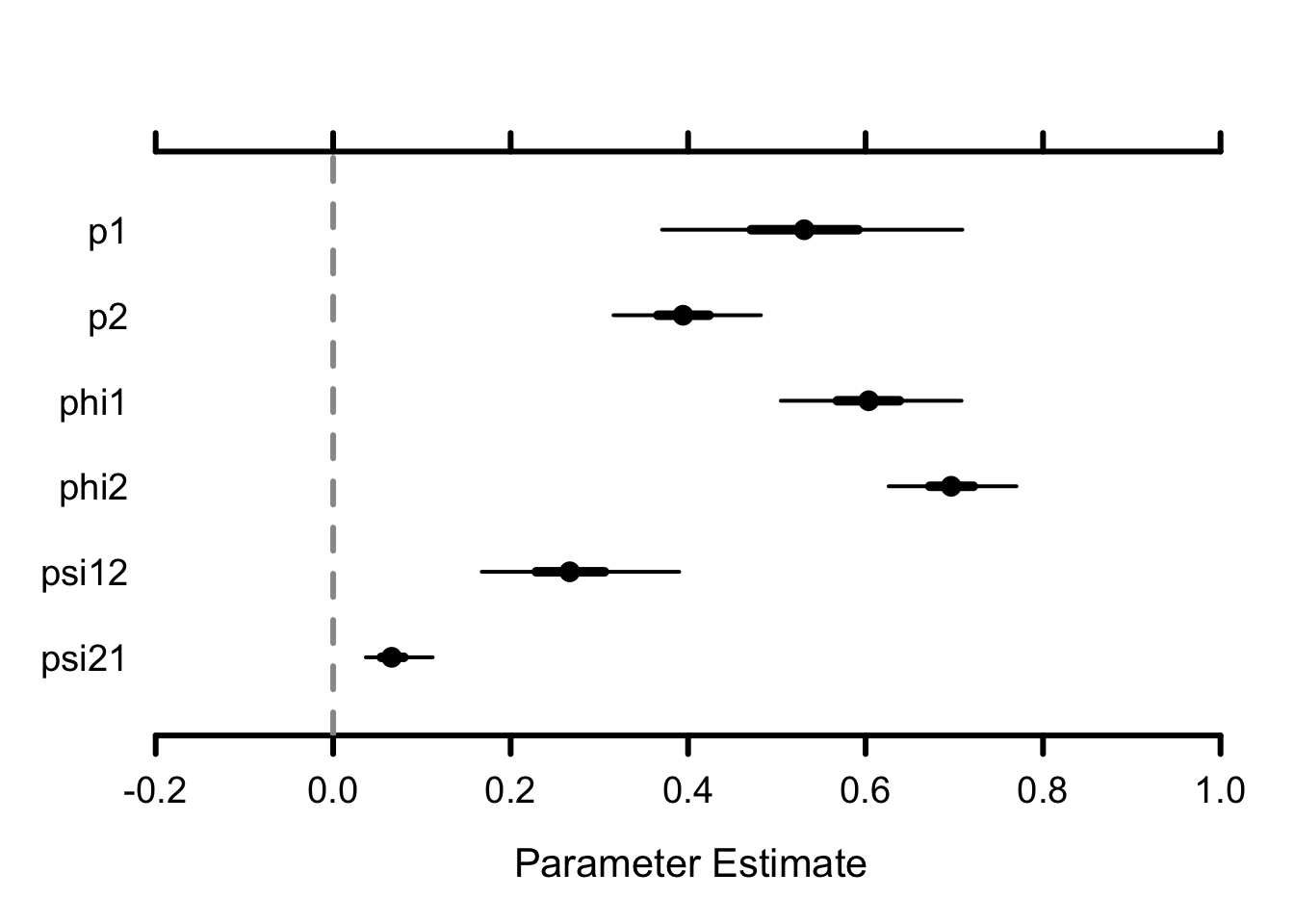

Remember mid–Atlantic is site 1, and Chesapeake site 2. Detection in mid–Atlantic (around 0.5) is higher than in Cheasapeake (around 0.4) although it comes with more uncertainty (wider credible interval). Survival in both sites are similar estimated at around 0.6–0.7. Note that by going multisite, we could make these parameters site-specific and differences might reflect habitat quality for example. Now the novelty lies in our capability to estimate movements from site 1 to site 2 and from site 2 to site 1 from a winter to the next. The annual probability of remaining in the same site for two successive winters, used as a measure of site fidelity, was lower in the mid–Atlantic (around 0.7) than in the Chesapeake (0.9). The estimated probability of moving to the Chesapeake from the mid–Atlantic was three times as high as the probability of moving in the opposite direction.

We may also have a look to numerical summaries, which confirm our ecological interpretation of the model parameter estimates:

MCMCsummary(mcmc.multisite, round = 2)
##       mean   sd 2.5%  50% 97.5% Rhat n.eff
## p1    0.56 0.10 0.37 0.56  0.76 1.00   157
## p2    0.40 0.04 0.32 0.39  0.48 1.00   217
## phi1  0.56 0.08 0.40 0.56  0.72 1.04   155
## phi2  0.72 0.05 0.63 0.72  0.83 1.02   120
## pi1   0.37 0.10 0.21 0.36  0.60 1.02    62
## psi12 0.23 0.09 0.08 0.22  0.43 1.03   171
## psi21 0.06 0.02 0.02 0.05  0.11 1.01   336

You could add time-dependence to the demographic parameters, e.g. survival and movements, and assess the effect of winter harshness with some temporal covariates. Individual covariates could also be considered.

Before we move to the next section, I will illustrate the use of nimbleEcology to fit the AS to the geese data with 2 sites (see Section 3.8.3). Using the function dHMM() which implements HMM with time-independent observation and transition matrices, we have:

# read in data
geese <- read_csv("geese.csv", col_names = TRUE)
y <- as.matrix(geese)
# drop Carolinas
y[y==3] <- 0 # act as if there was no detection in site 3 Carolinas
mask <- apply(y, 1, sum)
y <- y[mask!=0,] # remove rows w/ 0s only
# get occasions of first encounter
get.first <- function(x) min(which(x != 0))
first <- apply(y, 1, get.first)
# filter out individuals that are first captured at last occasion. 
# These individuals do not contribute to parameter estimation, 
# and also they cause problems with nimbleEcology
mask <- which(first!=ncol(y)) 
y <- y[mask, ]                # keep only these
first <- first[mask]

# NIMBLE code 
multisite.marginalized <- nimbleCode({
  
  # -------------------------------------------------
  # Parameters:
  # phi1: survival probability site 1
  # phi2: survival probability site 2
  # psi12: movement probability from site 1 to site 2
  # psi21: movement probability from site 2 to site 1
  # p1: recapture probability site 1
  # p2: recapture probability site 2
  # pi1: prop of being in site 1 at initial capture
  # -------------------------------------------------
  # States (z):
  # 1 alive at 1
  # 2 alive at 2
  # 3 dead
  # Observations (y):  
  # 1 not seen
  # 2 seen at site 1 
  # 3 seen at site 2
  # -------------------------------------------------
  
  # priors
  phi1 ~ dunif(0, 1)
  phi2 ~ dunif(0, 1)
  psi12 ~ dunif(0, 1)
  psi21 ~ dunif(0, 1)
  p1 ~ dunif(0, 1)
  p2 ~ dunif(0, 1)
  pi1 ~ dunif(0, 1)
  
  # probabilities of state z(t+1) given z(t)
  gamma[1,1] <- phi1 * (1 - psi12)
  gamma[1,2] <- phi1 * psi12
  gamma[1,3] <- 1 - phi1
  gamma[2,1] <- phi2 * psi21
  gamma[2,2] <- phi2 * (1 - psi21)
  gamma[2,3] <- 1 - phi2
  gamma[3,1] <- 0
  gamma[3,2] <- 0
  gamma[3,3] <- 1
  
  # probabilities of y(t) given z(t)
  omega[1,1] <- 1 - p1     # Pr(alive 1 t -> non-detected t)
  omega[1,2] <- p1        # Pr(alive 1 t -> detected 1 t)
  omega[1,3] <- 0          # Pr(alive 1 t -> detected 2 t)
  omega[2,1] <- 1 - p2     # Pr(alive 2 t -> non-detected t)
  omega[2,2] <- 0          # Pr(alive 2 t -> detected 1 t)
  omega[2,3] <- p2         # Pr(alive 2 t -> detected 2 t)
  omega[3,1] <- 1          # Pr(dead t -> non-detected t)
  omega[3,2] <- 0          # Pr(dead t -> detected 1 t)
  omega[3,3] <- 0          # Pr(dead t -> detected 2 t)
  
  # likelihood 
  # initial state probs
  for(i in 1:N) {
    init[i, 1:3] <- gamma[ y[i, first[i] ] - 1, 1:3 ] # first state propagation
  }
  for (i in 1:N){
    y[i,(first[i]+1):K] ~ dHMM(init = init[i,1:3],  # count data from first[i] + 1
                               probObs = omega[1:3,1:3],     # observation matrix
                               probTrans = gamma[1:3,1:3],   # transition matrix
                               len = K - first[i],           # nb of occasions
                               checkRowSums = 0)             # do not check whether elements in a row sum up to 1
  }
})
# constants
my.constants <- list(first = first, 
                     K = ncol(y), 
                     N = nrow(y))
# data
my.data <- list(y = y + 1)
# initial values 
initial.values <- function(){list(phi1 = runif(1, 0, 1), 
                                  phi2 = runif(1, 0, 1), 
                                  psi12 = runif(1, 0, 1), 
                                  psi21 = runif(1, 0, 1), 
                                  p1 = runif(1, 0, 1), 
                                  p2 = runif(1, 0, 1))}
# parameters to monitor
parameters.to.save <- c("phi1", "phi2","psi12", "psi21", "p1", "p2")
# MCMC details
n.iter <- 5000
n.burnin <- 1000
n.chains <- 2
# run NIMBLE
mcmc.multisite.marginalized <- nimbleMCMC(code = multisite.marginalized, 
                             constants = my.constants,
                             data = my.data,              
                             inits = initial.values,
                             monitors = parameters.to.save,
                             niter = n.iter,
                             nburnin = n.burnin, 
                             nchains = n.chains)

We obtain:

MCMCsummary(mcmc.multisite.marginalized, round = 2)
##       mean   sd 2.5%  50% 97.5% Rhat n.eff
## p1    0.53 0.09 0.36 0.53  0.71    1   651
## p2    0.40 0.04 0.32 0.39  0.49    1   618
## phi1  0.60 0.05 0.51 0.60  0.71    1   935
## phi2  0.70 0.04 0.63 0.70  0.76    1   804
## psi12 0.27 0.06 0.17 0.26  0.39    1   973
## psi21 0.07 0.02 0.04 0.07  0.11    1   965

There are slight differences in these parameters estimates compared to those we obtained earlier. This is probably due to the effective sample sizes being much bigger here (by a factor 3) with the marginalized likelihood for the same number of MCMC iterations.

5.3.3 Goodness of fit

Like for the CJS model, we need to ensure that the AS model provides a good fit to the data. To do so, both posterior predictive checks and classical procedures can be used. I illustrate the use of posterior predictive checks in Section 7.6. With regard to classical tests, the goodness-of-fit testing procedures we covered in Section 4.7 for the CJS model have been extended to the AS model. These procedure are also available in the package R2ucare. While the transience and trap-dependence tests can be used on each site, it is worth mentionning a test that is specific to the AS model with several sites. The “where before where after” (WBWA) tests for memory, in other words it’s a test for the Markovian property of the HMM in the particular context of capture-recapture. WBWA quantifies whether there is a relationship between where an animal has last been seen and where it will next be seen again. If a relationship exists, positive or negative, this suggests memory in the movements, and the probability for an animal of moving to a site at $t$, given it is present in a site at $t-1$ should be made dependent of where it was at $t-2$. This is called a second-order Markov process.

Going back to the geese data, the WBWA test is implemented as follows on the whole dataset:

library(R2ucare)
geese <- read_csv2("dat/allgeese.csv") %>% as.matrix()
y <- geese[,1:6]
size <- geese[,7]
wbwa <- test3Gwbwa(y, size)
wbwa$test3Gwbwa
##  stat    df p_val 
## 472.9  20.0   0.0

There is clearly a strong (not to say significant) positive relationship judging by the value of the statistic. I will demonstrate how to account for this memory issue in an extension of the AS model in a case study in Section 7.5.

5.4 What if more than 2 sites?

So far we have considered two sites only, for the sake of simplicity. Indeed when going for three sites (or more), a difficulty arises. While the movement probabilities still need to be between 0 and 1, the sum of all probabilities of moving from a site should also sum to one. This is because an individual alive in site 1 for example, has to stay in 1, move to 2 or move to 3, it has no other choice. This is no problem when you have only two sites because the probability of moving from 1 to 2 is always estimated between 0 and 1, and its complementary, the probability of moving from 2 to 1 will be too. When you have three sites, it might happen that the sum of the estimates for $\psi^{12}$ and $\psi^{13}$ is larger than one, even though they’re both between 0 and 1, which would make $\psi^{11} = 1 - \psi^{12} - \psi^{13}$ negative.

There are basically two methods to fulfill both constraints, either to assign a Dirichlet (which is pronounced deer-eesh-lay) prior to the movement probabilities, or to use a multinomial logit link function.

5.4.1 Dirichlet prior

The Dirichlet distribution extends the Beta distribution multivariate we have seen previously (Figure 1.2) for values between 0 and 1 that add up to 1. Going back to our example with 3 sites, we would like to come up with a prior for parameters of moving from 1, which are $\psi^{11}$, $\psi^{12}$ and $\psi^{13}$. The Dirichlet distribution of dimension 3 has a vector of parameters $(\alpha_1, \alpha_2, \alpha_3)$ that controls its shape. The sum of all $\alpha$’s can be interpreted as a measure of precision: The higher the sum, the more peaked is the distribution on the mean value, the mean value along each dimension being the ratio of the corresponding over the sum of all $\alpha$’s. When all $\alpha$’s are equal, the distribution is symmetric (Figure 5.2). Its mean is $(1/3, 1/3, 1/3)$ in our example with 3 parameters, whatever the value of $\alpha$. When $\alpha_1 = \alpha_2 = \alpha_3 = 1$, we obtain a uniform marginal distribution for the $\psi$’s, while values below 1 ($\alpha_1 = \alpha_2 = \alpha_3 = 0.1$) result in the distribution concentrating in the corners (skewed U-shaped forms) and values above 1 ($\alpha_1 = \alpha_2 = \alpha_3 = 10$) result in unimodal marginal distributions.

library(gtools) # to make the rdirichlet() function available
library(ggtern) # to visually represent multidim prob distribution 
set.seed(123) # for reproducibility
n <- 1000 # number of values drawn from Dirichlet distribution
alpha1 <- c(.1, .1, .1)
p1 <- rdirichlet(n, alpha1)
alpha2 <- c(1, 1, 1)
p2 <- rdirichlet(n, alpha2)
alpha3 <- c(10, 10, 10)
p3 <- rdirichlet(n, alpha3)
df <- cbind(rbind(p1, p2, p3), c(rep("alpha = c(0.1, 0.1, 0.1)", n),
                                     rep("alpha = c(1, 1, 1)", n),
                                     rep("alpha = c(10, 10, 10)", n))) %>%
  as_tibble() %>%
  mutate(x = as.numeric(V1),
         y = as.numeric(V2),
         z = as.numeric(V3),
         alpha = V4)

df %>%
  ggtern(aes(x = x, y = y, z = z)) +
  stat_density_tern(aes(fill=..level.., alpha=..level..),
                    geom = 'polygon',
                    bdl = 0.005) + # a 2D kernel density estimation of the distribution
  scale_fill_viridis_b() +
  geom_point(alpha = 0.3, pch = "+") +
  theme_showarrows() +
  scale_T_continuous(breaks = seq(0, 1, by = 0.2),
                     labels = seq(0, 1, by = 0.2)) +
  scale_L_continuous(breaks = seq(0, 1, by = 0.2),
                     labels = seq(0, 1, by = 0.2)) +
  scale_R_continuous(breaks = seq(0, 1, by = 0.2),
                     labels = seq(0, 1, by = 0.2)) +
  labs(x = "",
       y = "",
       z = "",
       Tarrow = "psi11",
       Larrow = "psi12",
       Rarrow = "psi13") +
  guides(color = "none", fill = "none", alpha = "none") +
  facet_wrap(~alpha, ncol = 3)

$The Dirichlet distribution as a prior for $(\psi^{11}, \psi^{12}, \psi^{13})$ with vector of parameters $\alpha$. Here all components of $\alpha$ are equal which makes the distribution symmetric, and its mean is $(1/3, 1/3, 1/3)$. When $\alpha = 1$, the prior for the $\psi$’s is uniform (middle panel), unimodal when $\alpha = 10$ (right panel) and concentrated in the corners (0 and 1) when $\alpha = 0.1$ (left panel).$

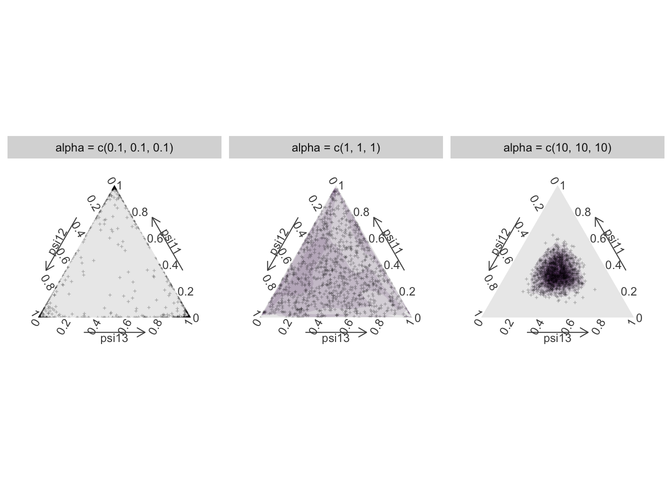
Figure 5.2: The Dirichlet distribution as a prior for $(\psi^{11}, \psi^{12}, \psi^{13})$ with vector of parameters $\alpha$. Here all components of $\alpha$ are equal which makes the distribution symmetric, and its mean is $(1/3, 1/3, 1/3)$. When $\alpha = 1$, the prior for the $\psi$’s is uniform (middle panel), unimodal when $\alpha = 10$ (right panel) and concentrated in the corners (0 and 1) when $\alpha = 0.1$ (left panel).

Going back to our example, in NIMBLE, we consider a Dirichlet prior for each triplet of movement parameters, from site 1 ($\psi^{11}$, $\psi^{12}$ and $\psi^{13}$), from site 2 ($\psi^{21}$, $\psi^{22}$ and $\psi^{23}$) and from site 3 ($\psi^{31}$, $\psi^{32}$ and $\psi^{33}$).

We start by setting the scene with comments:

...
  # -------------------------------------------------
  # Parameters:
  # phi1: survival probability site 1
  # phi2: survival probability site 2
  # phi3: survival probability site 3
  # psi11 = psi1[1]: movement probability from site 1 to site 1 (reference)
  # psi12 = psi1[2]: movement probability from site 1 to site 2
  # psi13 = psi1[3]: movement probability from site 1 to site 3 
  # psi21 = psi2[1]: movement probability from site 2 to site 1
  # psi22 = psi2[2]: movement probability from site 2 to site 2 (reference)
  # psi23 = psi2[3]: movement probability from site 2 to site 3
  # psi31 = psi3[1]: movement probability from site 3 to site 1
  # psi32 = psi3[2]: movement probability from site 3 to site 2
  # psi33 = psi3[3]: movement probability from site 3 to site 3 (reference)
  # p1: recapture probability site 1
  # p2: recapture probability site 2
  # p3: recapture probability site 3
  # -------------------------------------------------
  # States (z):
  # 1 alive at 1
  # 2 alive at 2
  # 2 alive at 3
  # 3 dead
  # Observations (y):  
  # 1 not seen
  # 2 seen at 1 
  # 3 seen at 2
  # 3 seen at 3
...

multisite <- nimbleCode({
...
  # transitions: Dirichlet priors
  psi1[1:3] ~ ddirch(alpha[1:3]) # psi11, psi12, psi13
  psi2[1:3] ~ ddirch(alpha[1:3]) # psi21, psi22, psi23
  psi3[1:3] ~ ddirch(alpha[1:3]) # psi31, psi32, psi33
...

Then we use these parameters (which now respect the constraints) to define the transition matrix:

multisite <- nimbleCode({
...
  # probabilities of state z(t+1) given z(t)
  gamma[1,1] <- phi1 * psi1[1]
  gamma[1,2] <- phi1 * psi1[2]
  gamma[1,3] <- phi1 * psi1[3]
  gamma[1,4] <- 1 - phi1
  gamma[2,1] <- phi2 * psi2[1]
  gamma[2,2] <- phi2 * psi2[2]
  gamma[2,3] <- phi2 * psi2[3]
  gamma[2,4] <- 1 - phi2
  gamma[3,1] <- phi3 * psi3[1]
  gamma[3,2] <- phi3 * psi3[2]
  gamma[3,3] <- phi3 * psi3[3]
  gamma[3,4] <- 1 - phi3
  gamma[4,1] <- 0
  gamma[4,2] <- 0
  gamma[4,3] <- 0
  gamma[4,4] <- 1
...

When we fit this model to the geese dataset with the detections in the Carolinas wintering site back in, and with alpha <- c(1, 1, 1) passed to the constants, we obtain the following results:

MCMCsummary(mcmc.multisite, round = 2)
##         mean   sd 2.5%  50% 97.5% Rhat n.eff
## p1      0.51 0.08 0.36 0.51  0.67 1.02   306
## p2      0.45 0.05 0.36 0.45  0.55 1.00   217
## p3      0.26 0.06 0.15 0.25  0.39 1.01   166
## phi1    0.60 0.05 0.51 0.60  0.70 1.01   384
## phi2    0.70 0.04 0.63 0.70  0.77 1.00   233
## phi3    0.75 0.06 0.62 0.76  0.87 1.03   218
## psi1[1] 0.74 0.05 0.63 0.75  0.84 1.01   818
## psi1[2] 0.24 0.05 0.14 0.24  0.35 1.02   817
## psi1[3] 0.02 0.02 0.00 0.01  0.07 1.05   487
## psi2[1] 0.07 0.02 0.04 0.07  0.12 1.00   668
## psi2[2] 0.84 0.04 0.75 0.84  0.90 1.00   292
## psi2[3] 0.09 0.03 0.04 0.08  0.17 1.00   220
## psi3[1] 0.02 0.01 0.00 0.02  0.06 1.00  1022
## psi3[2] 0.22 0.05 0.12 0.21  0.33 1.01   525
## psi3[3] 0.76 0.06 0.64 0.76  0.86 1.01   506

Survival probabilities are similar among sites, but the detection probability in Carolinas seems much lower than in the two other wintering sites. The estimated probability of moving to the Chesapeake from the Carolinas is 2 times as high as the probability of moving in the opposite direction.

In theory, you could include covariates as in 4.8 through the $\alpha$ parameters and the use a log link function (to ensure $\alpha > 0$), e.g. $\log(\alpha) = \beta_1 + \beta_2 x$. However, NIMBLE does not allow that. Fortunately, there is another way to specify the Dirichlet distribution through a ratio of gamma distributions that allows to incorporate covariates.

The gamma distribution is continuous. It has two parameters $\alpha$ and $\theta$ that control its shape and scale (Figure 5.3). Another parameterization considers its shape and rate which is the inverse of the scale.

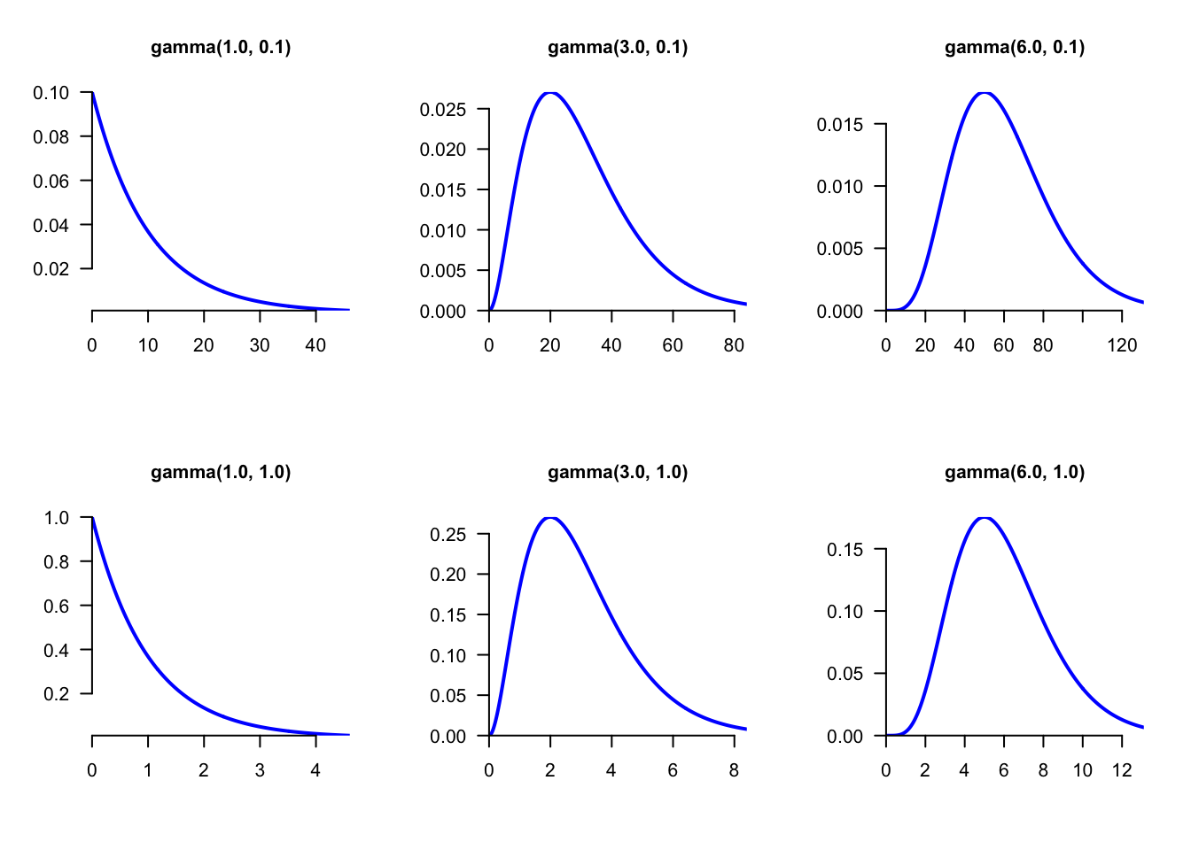
$The distribution gamma($\alpha$,$\theta$) for different values of $\alpha$ and $\theta$. The shape argument $\alpha$ determines the overall shape while the scale parameter $\theta$ only affects the scale values (compare the values on X- and Y-axes between the bottom and upper panels). The exponential and chi-square distributions are particular cases of the gamma distribution. If the parameter shape is close to zero, the gamma is very similar to the exponential (bottom and upper left panels). If the parameter shape is large, then the gamma is similar to the chi-squared distribution (bottom and upper right panels).$

Figure 5.3: The distribution gamma($\alpha$,$\theta$) for different values of $\alpha$ and $\theta$. The shape argument $\alpha$ determines the overall shape while the scale parameter $\theta$ only affects the scale values (compare the values on X- and Y-axes between the bottom and upper panels). The exponential and chi-square distributions are particular cases of the gamma distribution. If the parameter shape is close to zero, the gamma is very similar to the exponential (bottom and upper left panels). If the parameter shape is large, then the gamma is similar to the chi-squared distribution (bottom and upper right panels).

If we have three independent random variables $Y_1, Y_2$ and $Y_3$ distributed as gamma distributions with shape parameters the $\alpha$’s and same scale parameter $\theta$, that is $Y_j \sim \text{Gamma}(\alpha_j, \theta)$, then it can be shown that the vector $(Y_1/V, Y_2/V, Y_3/V)$ is Dirichlet with vector of parameters the $\alpha$’s, where $V$ is the sum of the $Y$’s (which is also gamma distributed). In NIMBLE, this suggests using $\theta = 1$ to get a uniform prior:

...
# transitions: Dirichlet priors with Gamma formulation
for (s in 1:3){
  lpsi1[s] ~ dgamma(alpha[s], 1) # Y1, Y2, Y3 for psi11, psi12, psi13
  psi1[s] <- lpsi1[s]/V1 # psi11, psi12, psi13
  lpsi2[s] ~ dgamma(alpha[s], 1) # Y'1, Y'2, Y'3 for psi21, psi22, psi23
  psi2[s] <- lpsi2[s]/V2 # psi21, psi22, psi23
  lpsi3[s] ~ dgamma(alpha[s], 1) # Y''1, Y''2, Y''3 for psi31, psi32, psi33
  psi3[s] <- lpsi3[s]/V3 # psi31, psi32, psi33
}
V1 <- sum(lpsi1[1:3])
V2 <- sum(lpsi2[1:3])
V3 <- sum(lpsi3[1:3])
...

From there, we can express the shape parameter of the gamma distribution (precisely the $\alpha$’s here) as a function of covariates as in $\log(\alpha) = \beta_1 + \beta_2 x$ in the spirit of a generalized linear model with a gamma response.

5.4.2 Multinomial logit

Another possibility to build a prior that ensures the movement probabilities are between 0 and 1 and sum up to 1 is to extend the logit link we used for the CJS model in Section 4.8. Remember we had $\text{logit}(\phi) = \beta$, we specified a prior on $\beta$ say $\beta \sim N(0,1.5)$ then got a prior on $\phi$ by back-transforming $\beta$ with $\phi = \text{logit}^{-1}(\beta)$.

Going back to our example with $3$ sites, and focusing on the movement probabilities say, from site 1, we first choose a reference (or pivot) site, say 1, then $\log\left(\displaystyle{\frac{\psi^{12}}{\psi^{11}}}\right) = \beta_2$ and $\log\left(\displaystyle{\frac{\psi^{13}}{\psi^{11}}}\right) = \beta_3$. Interestingly, when exponentiated, the $\beta$’s here can be interpreted as the increase in the odds of moving versus staying on site resulting from a one-unit increase in the covariate. Any of the sites can be chosen to be the reference, this will not change the likelihood and you will get the same results. Now we specify a normal prior distribution for the $\beta$’s. Eventually, to back-transform, we use $\psi^{12} = \displaystyle{\frac{\exp(\beta_2)}{1+\displaystyle{\exp(\beta_2)+\displaystyle{\exp(\beta_3)}}}}$ and $\psi^{13} = \displaystyle{\frac{\exp(\beta_3)}{1+\displaystyle{\exp(\beta_2)+\displaystyle{\exp(\beta_3)}}}}$. The reference parameter, here $\psi^{11}$, is calculated as $\psi^{11} = \displaystyle{\frac{1}{1 + \displaystyle{\exp(\beta_2)+\displaystyle{\exp(\beta_3)}}}}$, or simply as the complementary probability $\psi^{11} = 1 - \psi^{12} - \psi^{13}$.

Note that when there are only 2 sites instead of 3 or more, then the multinomial logit reduces to the logit link.

In NIMBLE, we write:

multisite <- nimbleCode({
...
  # transitions: multinomial logit
  for (i in 1:2){
    # normal priors on logit of all but one movement prob
    beta1[i] ~ dnorm(0, sd = 1.5)
    beta2[i] ~ dnorm(0, sd = 1.5)
    beta3[i] ~ dnorm(0, sd = 1.5)
    # constrain the transitions such that their sum is < 1
    psi1[i] <- exp(beta1[i]) / (1 + exp(beta1[1]) + exp(beta1[2]))
    psi2[i] <- exp(beta2[i]) / (1 + exp(beta2[1]) + exp(beta2[2]))
    psi3[i] <- exp(beta3[i]) / (1 + exp(beta3[1]) + exp(beta3[2]))
  }
  # reference movement probability
  psi1[3] <- 1 - psi1[1] - psi1[2]
  psi2[3] <- 1 - psi2[1] - psi2[2]
  psi3[3] <- 1 - psi3[1] - psi3[2]
...

Then we use these parameters (which now respect the constraints) to define the transition matrix:

multisite <- nimbleCode({
...
  # probabilities of state z(t+1) given z(t)
  gamma[1,1] <- phi1 * psi1[1]
  gamma[1,2] <- phi1 * psi1[2]
  gamma[1,3] <- phi1 * psi1[3]
  gamma[1,4] <- 1 - phi1
  gamma[2,1] <- phi2 * psi2[1]
  gamma[2,2] <- phi2 * psi2[2]
  gamma[2,3] <- phi2 * psi2[3]
  gamma[2,4] <- 1 - phi2
  gamma[3,1] <- phi3 * psi3[1]
  gamma[3,2] <- phi3 * psi3[2]
  gamma[3,3] <- phi3 * psi3[3]
  gamma[3,4] <- 1 - phi3
  gamma[4,1] <- 0
  gamma[4,2] <- 0
  gamma[4,3] <- 0
  gamma[4,4] <- 1
...

You may check that the results are very similar to those we obtained with the Dirichlet prior:

MCMCsummary(mcmc.multisite, round = 2)
##         mean   sd 2.5%  50% 97.5% Rhat n.eff
## p1      0.52 0.08 0.37 0.52  0.69 1.01   297
## p2      0.46 0.05 0.37 0.45  0.57 1.13   209
## p3      0.23 0.06 0.14 0.23  0.36 1.05   137
## phi1    0.60 0.05 0.50 0.60  0.70 1.00   403
## phi2    0.70 0.04 0.63 0.70  0.77 1.14   281
## phi3    0.77 0.06 0.64 0.77  0.89 1.05   199
## psi1[1] 0.74 0.06 0.62 0.74  0.83 1.00   727
## psi1[2] 0.22 0.05 0.13 0.22  0.33 1.03   795
## psi1[3] 0.04 0.03 0.01 0.04  0.12 1.05    88
## psi2[1] 0.07 0.02 0.04 0.07  0.11 1.01   655
## psi2[2] 0.83 0.04 0.74 0.84  0.90 1.04   153
## psi2[3] 0.10 0.04 0.04 0.09  0.19 1.03   122
## psi3[1] 0.03 0.02 0.01 0.02  0.07 1.01   794
## psi3[2] 0.22 0.05 0.13 0.21  0.32 1.02   477
## psi3[3] 0.76 0.05 0.64 0.76  0.85 1.02   444

Both the Dirichlet prior and the multinomial logit link give the same results, and there is not much difference in terms of runtime or quality of convergence, so you should use the option you feel the most comfortable with.

5.5 Sites may be states

So far, we have considered geographical locations (or sites) to refine the alive information when an animal is detected. However, it was quickly realized that sites could actually be states defined by physiology or behavior, hence opening up an avenue for applications of capture-recapture models in many fields of ecology.

Examples of states include:

Epidemiological or disease states: sick/healthy, uninfected/infected/recovered;
Morphological states: small/medium/big, light/medium/heavy;
Life-history states: e.g. breeder/non-breeder, failed breeder, first-time breeder;
Developmental states: e.g. juvenile/subadult/adult;
Social states: e.g. solitary/group-living, subordinate/dominant;
Death states: e.g. alive, dead from harvest, dead from natural causes.

In brief, states are individual, time-specific discrete covariates.

5.5.1 Titis data

To illustrate this section, we will consider data collected between 1942 and 1956 by Lance Richdale on the Sooty shearwaters (Ardenna grisea), also known as titis (Figure 5.4).

Figure 5.4: Sooty shearwater (Ardenna grisea). Credit: John Harrison.

You may see the data below:

titis <- read_csv2("dat/titis.csv", 
                   col_names = FALSE)
titis %>%
  rename(year_1942 = X1,
         year_1943 = X2,
         year_1944 = X3,
         year_1949 = X4,
         year_1952 = X5,
         year_1953 = X6,
         year_1956 = X7)
## # A tibble: 1,013 × 7
##    year_1942 year_1943 year_1944 year_1949 year_1952
##        <dbl>     <dbl>     <dbl>     <dbl>     <dbl>
##  1         0         0         0         0         0
##  2         0         0         0         0         0
##  3         0         0         0         0         0
##  4         0         0         0         0         0
##  5         0         0         0         0         0
##  6         0         0         0         0         0
##  7         0         0         0         0         0
##  8         0         0         0         0         0
##  9         0         0         0         0         0
## 10         0         0         0         0         0
## # ℹ 1,003 more rows
## # ℹ 2 more variables: year_1953 <dbl>, year_1956 <dbl>

In total, 1013 titis were captured, marked and recaptured on a small colony on Whero Island in southern New Zealand. These data were previously analyzed by Richard Scofield who kindly provided us with the data.

Following the way the data were collected, four states were originally considered: Alive breeder; Accompanied by another bird in a burrow; Alone in a burrow; On the surface; Dead. For simplicity, we pooled all alive states (except breeder) together in a non-breeder state (NB) that includes failed breeders (birds that had bred previously – skip reproduction or divorce) and pre-breeders (birds that had yet to breed). Because burrows were not checked before hatching, some birds in the category NB might have already failed. Therefore birds in the breeder state (B) should be seen as successful breeders, and those in the NB state as nonbreeders plus prebreeders and failed breeders.

In summary, we code the states as 1 for alive and breeding, 2 for alive and non-breeding and 3 for dead. To make the modelling process more self-explanatory, we will use letters B, NB and D but you should keep in mind that these are actually numbers. Observations are non-detected coded as 1, and detected as breeder or non-breeder coded as 2 and 3 respectively.

The aim here is to study life-history trade–offs. Specifically, we ask the questions: Does breeding affect survival? Does breeding in current year affect breeding next year?

5.5.2 The AS model for states

Basically, the AS model with states is the same model as in the geese example with two sites, see Sections 5.2 and 5.3.

If we let $\phi^B$ and $\phi^{NB}$ be the survival probabilities of breeders and non-breeders, $\psi^{NBB}$ the probability of becoming breeder for a non-breeder, and $\psi^{BNB}$ the probability of skipping reproduction, then the transition matrix is:

\[\begin{matrix} & \\ \mathbf{\Gamma} = \left ( \vphantom{ \begin{matrix} 12 \\ 12 \\ 12 \end{matrix} } \right . \end{matrix} \hspace{-1.2em} \begin{matrix} z_t=B & z_t=NB & z_t=D \\ \hdashline \phi^B (1-\psi^{BNB}) & \phi^B \psi^{BNB} & 1 - \phi^B\\ \phi^{NB} \psi^{NBB} & \phi^{NB} (1-\psi^{NBB}) & 1 - \phi^{NB}\\ 0 & 0 & 1 \end{matrix} \hspace{-0.2em} \begin{matrix} & \\ \left . \vphantom{ \begin{matrix} 12 \\ 12 \\ 12 \end{matrix} } \right ) \begin{matrix} z_{t-1}=B \\ z_{t-1}=NB \\ z_{t-1}=D \end{matrix} \end{matrix}\]

The costs or reproduction would reflect in future reproduction if breeders have a lower probability of breed next year than non-breeders $\psi^{BB} = 1 - \psi^{BNB} < \psi^{NBB}$ or in survival if the survival of breeders is lower than that of non-breeders $\phi^B < \phi^{NB}$.

The observation matrix is:

\[\begin{matrix} & \\ \mathbf{\Omega} = \left ( \vphantom{ \begin{matrix} 12 \\ 12 \\ 12 \end{matrix} } \right . \end{matrix} \hspace{-1.2em} \begin{matrix} y_t=1 & y_t=2 & y_t=3 \\ \hdashline 1 - p^B & p^B & 0\\ 1 - p^{NB} & 0 & p^{NB}\\ 1 & 0 & 0 \end{matrix} \hspace{-0.2em} \begin{matrix} & \\ \left . \vphantom{ \begin{matrix} 12 \\ 12 \\ 12 \end{matrix} } \right ) \begin{matrix} z_{t}=B \\ z_{t}=NB \\ z_{t}=D \end{matrix} \end{matrix}\]

where $p^B$ and $p^{NB}$ are the detection proabilities of non-breeders and breeders respectively.

5.5.3 NIMBLE implementation

We first write the NIMBLE code, which is exactly the same as in the geese example with two sites, see Section 5.3.

First some definitions which we have as comments in the code:

multistate <- nimbleCode({
  # -------------------------------------------------
  # Parameters:
  # B is for breeder, NB for non-breeder
  # phiB: survival probability state B
  # phiNB: survival probability state NB
  # psiBNB: transition probability from B to NB
  # psiNBB: transition probability from NB to B
  # pB: detection probability B
  # pNB: detection probability NB
  # -------------------------------------------------
  # States (z):
  # 1 alive B
  # 2 alive NB
  # 3 dead
  # Observations (y):
  # 1 not seen
  # 2 seen as B
  # 3 seen as NB
  # -------------------------------------------------
...

Then the priors:

multistate <- nimbleCode({
...
  # Priors
  phiB ~ dunif(0, 1)
  phiNB ~ dunif(0, 1)
  psiBNB ~ dunif(0, 1)
  psiNBB ~ dunif(0, 1)
  pB ~ dunif(0, 1)
  pNB ~ dunif(0, 1)
...

The transition matrix:

multistate <- nimbleCode({
...
  # probabilities of state z(t+1) given z(t)
  gamma[1,1] <- phiB * (1 - psiBNB)
  gamma[1,2] <- phiB * psiBNB
  gamma[1,3] <- 1 - phiB
  gamma[2,1] <- phiNB * psiNBB
  gamma[2,2] <- phiNB * (1 - psiNBB)
  gamma[2,3] <- 1 - phiNB
  gamma[3,1] <- 0
  gamma[3,2] <- 0
  gamma[3,3] <- 1
...

The observation matrix:

multistate <- nimbleCode({
...
  # probabilities of y(t) given z(t)
  omega[1,1] <- 1 - pB    # Pr(alive B t -> non-detected t)
  omega[1,2] <- pB        # Pr(alive B t -> detected B t)
  omega[1,3] <- 0         # Pr(alive B t -> detected NB t)
  omega[2,1] <- 1 - pNB   # Pr(alive NB t -> non-detected t)
  omega[2,2] <- 0         # Pr(alive NB t -> detected B t)
  omega[2,3] <- pNB       # Pr(alive NB t -> detected NB t)
  omega[3,1] <- 1         # Pr(dead t -> non-detected t)
  omega[3,2] <- 0         # Pr(dead t -> detected N t)
  omega[3,3] <- 0         # Pr(dead t -> detected NB t)
...

And the likelihood:

multistate <- nimbleCode({
...
  # likelihood
  for (i in 1:N){
    # latent state at first capture
    z[i,first[i]] <- y[i,first[i]] - 1
    for (t in (first[i]+1):K){
      # z(t) given z(t-1)
      z[i,t] ~ dcat(gamma[z[i,t-1],1:3])
      # y(t) given z(t)
      y[i,t] ~ dcat(omega[z[i,t],1:3])
    }
  }
})

We run NIMBLE and get the following results:

MCMCsummary(mcmc.multistate, round = 2)
##        mean   sd 2.5%  50% 97.5% Rhat n.eff
## pB     0.60 0.03 0.54 0.59  0.66 1.00   202
## pNB    0.57 0.03 0.51 0.57  0.62 1.01   281
## phiB   0.80 0.02 0.77 0.80  0.83 1.01   313
## phiNB  0.85 0.02 0.82 0.85  0.88 1.00   404
## psiBNB 0.25 0.02 0.21 0.25  0.30 1.00   434
## psiNBB 0.24 0.02 0.20 0.24  0.29 1.03   478

Non-breeder individuals seem to have a survival higher than breeder individuals, suggesting a trade-off between reproduction and survival. Let’s compare graphically the survival of breeder and non-breeder individuals. First we gather the values generated for $\phi^B$ and $\phi^{NB}$ for the two chains:

phiB <- c(mcmc.multistate$chain1[,"phiB"], mcmc.multistate$chain2[,"phiB"])
phiNB <- c(mcmc.multistate$chain1[,"phiNB"], mcmc.multistate$chain2[,"phiNB"])
df <- data.frame(param = c(rep("phiB", length(phiB)), 
                           rep("phiNB", length(phiB))), 
                 value = c(phiB, phiNB))

Then, we plot the two posterior distributions:

df %>%
  ggplot(aes(x = value, fill = param)) +
  geom_density(color = "white", alpha = 0.6, position = 'identity') +
  scale_fill_manual(values = c("#69b3a2", "#404080")) +
  labs(fill = "", x = "survival")

There is little overlap between the two distributions, suggesting an actual trade–off. A formal test of the trade-off would consist in fitting the model with survival irrespective of the state, and compare its WAIC value to the model we just fitted.

What about a potential trade-off on reproduction?

psiBNB <- c(mcmc.multistate$chain1[,"psiBNB"], mcmc.multistate$chain2[,"psiBNB"])
psiBB <- 1 - psiBNB
psiNBB <- c(mcmc.multistate$chain1[,"psiNBB"], mcmc.multistate$chain2[,"psiNBB"])
df <- data.frame(param = c(rep("psiBB", length(phiB)), 
                           rep("psiNBB", length(phiB))), 
                 value = c(psiBB, psiNBB))
df %>%
  ggplot(aes(x = value, fill = param)) +
  geom_density(color = "white", alpha = 0.6, position = 'identity') +
  scale_fill_manual(values = c("#69b3a2", "#404080")) +
  labs(fill = "", x = "breeding probabilities")

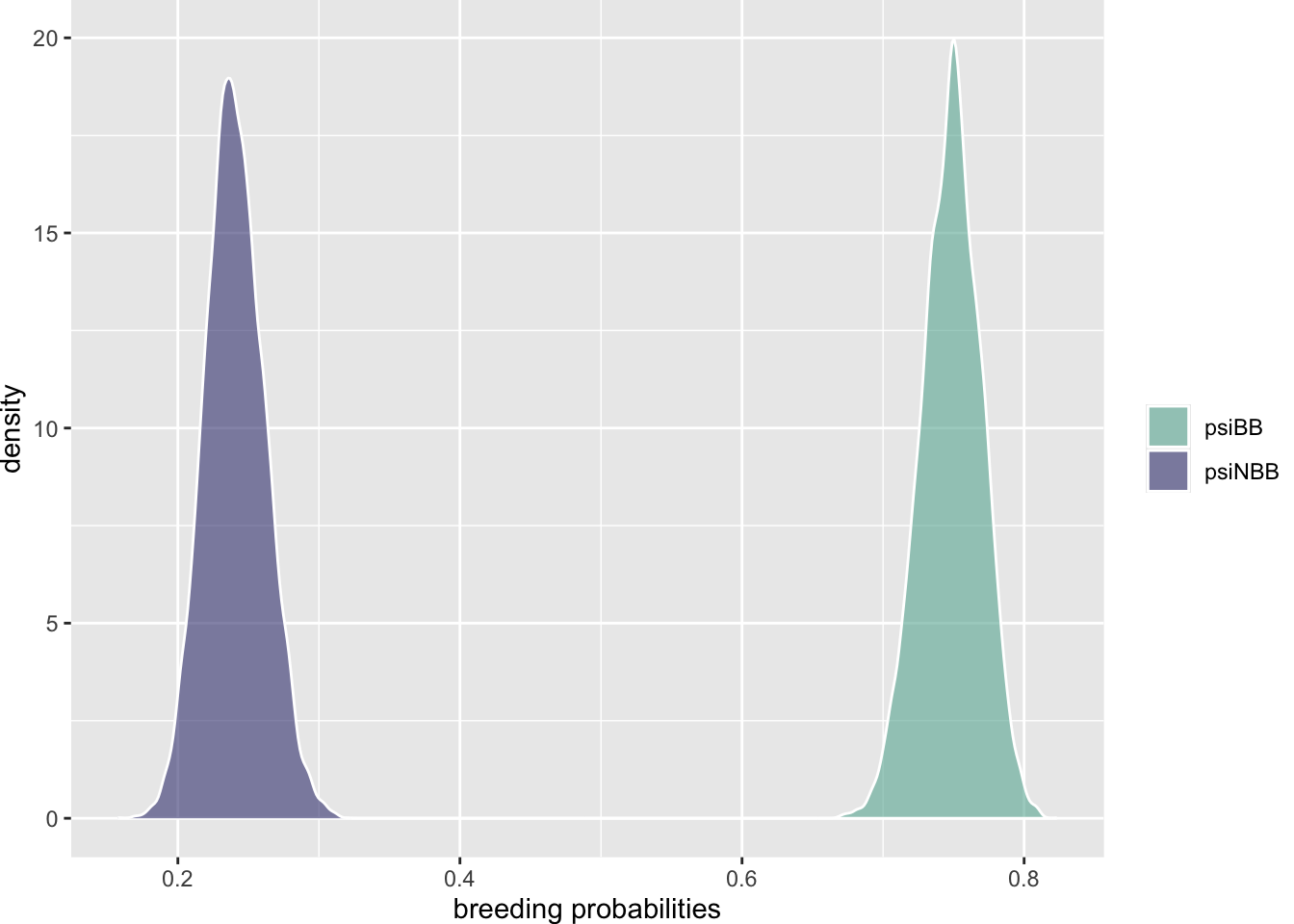
There is no overlap whatsoever, so the two transition probabilities are clearly different. Interestingly, breeder individuals do much better than non-breeder individuals. This failure at detecting a trade-off is probably due to individual heterogeneity that should be accounted for. We will do just that in a case study in Section 8.2.

5.6 Issue of local minima

In the frequentist approach, we use the maximum likelihood theory to estimate parameters. The maximum likelihood estimates are the values that get you to the maximum of the model likelihood. To find out the maximum of the likelihood, we use iterative optimization algorithms (e.g. the default method is that of Nelder and Mead in the R optim() function). However, sometimes, our model likelihood contains several maxima and there is no guarantee that the algorithms will find the global maximum corresponding to the maximum likelihood estimates, and it may get stuck in a local maximum. Let’s illustrate this issue with some simulated data that were kindly provided by Jérôme Dupuis. We consider 2 sites (or alive states), say 1 and 2, and 7 sampling occasions. The survival probability is constant $\phi = 1$ as well as the detection probability $p = 0.6$. The probability of moving from 1 to 2 is $\psi^{12} = 0.6$ and $\psi^{21} = 0.85$ in the opposite direction. Here are the encounter histories of the 27 individuals that were simulated by Jérôme:

dat <- matrix(c(2, 0, 2, 1, 2, 0, 2,
                2, 0, 2, 1, 2, 0, 2,
                2, 0, 2, 1, 2, 0, 2,
                2, 0, 2, 1, 2, 0, 2,
                1, 1, 1, 0, 1, 0, 1,
                1, 1, 1, 0, 1, 0, 1,
                1, 1, 1, 0, 1, 0, 1,
                1, 1, 1, 0, 1, 0, 1,
                2, 0, 2, 0, 2, 0, 1,
                2, 0, 2, 0, 2, 0, 1,
                2, 0, 2, 0, 2, 0, 1,
                2, 0, 2, 0, 2, 0, 1,
                1, 0, 1, 0, 1, 0, 1,
                1, 0, 1, 0, 1, 0, 1,
                1, 0, 1, 0, 1, 0, 1,
                1, 0, 1, 0, 1, 0, 1,
                2, 0, 2, 0, 2, 0, 2,
                2, 0, 2, 0, 2, 0, 2,
                2, 0, 2, 0, 2, 0, 2,
                2, 0, 2, 0, 2, 0, 2,
                1, 0, 1, 0, 1, 0, 2,
                1, 0, 1, 0, 1, 0, 2,
                1, 0, 1, 0, 1, 0, 2,
                1, 0, 1, 0, 1, 0, 2,
                2, 2, 0, 1, 0, 2, 1,
                2, 2, 0, 1, 0, 2, 1,
                2, 2, 0, 1, 0, 2, 1,
                2, 2, 0, 1, 0, 2, 1,
                2, 1, 0, 2, 0, 1, 1,
                2, 1, 0, 2, 0, 1, 1,
                2, 1, 0, 2, 0, 1, 1,
                2, 1, 0, 2, 0, 1, 1),
              byrow = T,
              ncol = 7)

In Figure 5.5, we provide an illustration of the influence of the choice of initial values when trying to maximize the likelihood, or rather to minimize the deviance (which is minus two times the log of the likelihood). The black curve is the what we called the profile deviance for $\psi^{21}$. Profiling the deviance consists in taking a slice of it in the direction of a parameter of interest and treating the other parameters as nuisance parameters. In our example, we set $\psi^{21}$ to a value (on the x-axis) an minimize the deviance (on the y-axis) with respect to the other parameters. There are two minima, but only the global minimum (corresponding to the lowest value of deviance) corresponding to $\psi^{21}$ around 0.8 is of interest to us. The thing is that if you start your optimization algorithm by picking value in the red area, then it will get stuck in the local minimum and will tell you the maximum likelihood estimate of $\psi^{21}$ is around 0.35, which is obviously far from the value we used to simulate the data. In contrast, if you pick initial values in the green area, then the algorithm will converge to the global minimum.

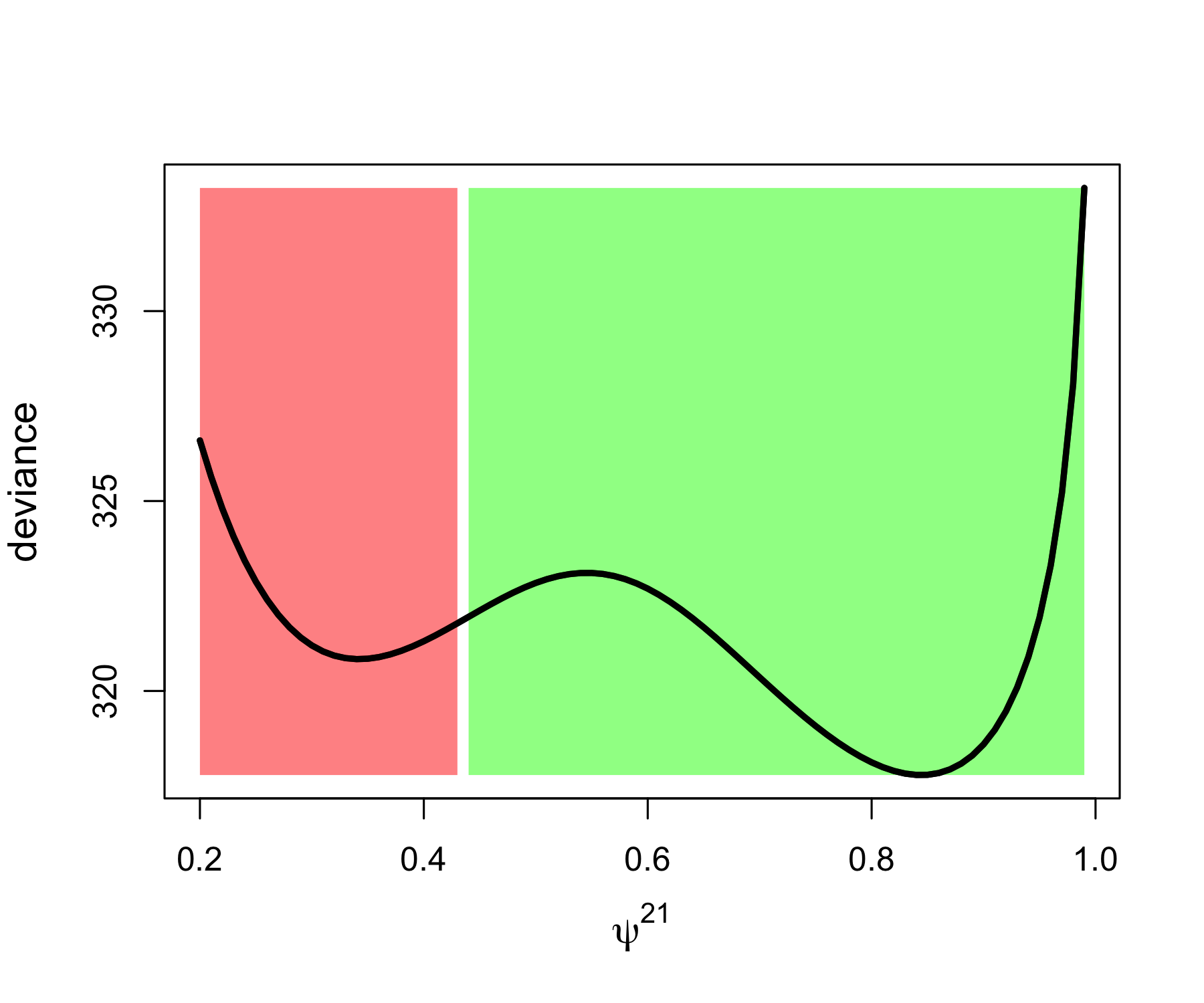
Figure 5.5: Influence of the choice of initial values on the convergence to the global minimum of the deviance illustrated with simulated data. The black curve is the profile deviance of the probability to move from site 2 to 1. If an initial value is picked in the red area, we end up in the local minimum while if it is picked in the green area, then we get the global minimum which corresponds to the maximum lilkelihood estimate.

You might argue that this is a problem of the optimization algorithm and therefore inherent to the frequentist approach. Well, it turns out that MCMC algorithms are not immune to the issue. If you fit the AS model with constant parameters to the simulated data, here is the trace for the probability of moving from 2 to 1:

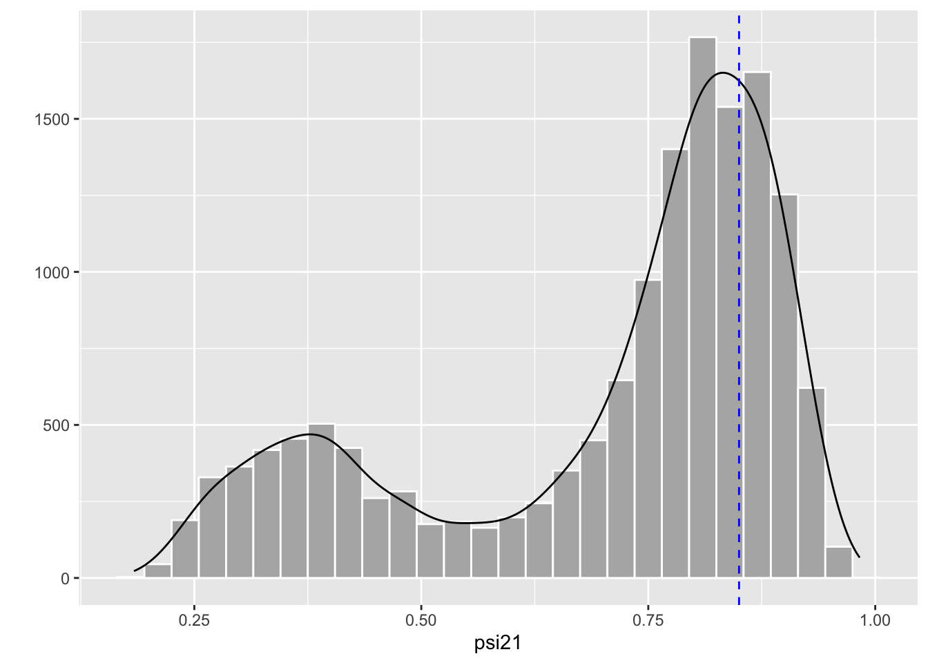
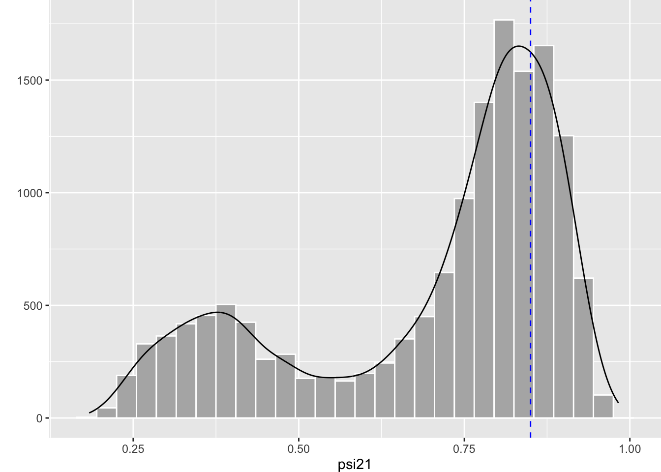
Clearly, there are two regimes. The chain spends most of its time around high values of $\psi^{21}$ close to the true value represented by the blue dashed line. But sometimes, the chain jumps to values around 0.3-0.4. This behavior translates into two modes in the posterior distribution for $\psi^{21}$ where the mode on the right is closer to the truth represented by the dashed blue vertical line:

The issue of local minima is a difficult problem. How to get out of this problematic situation? In the frequentist approach, the trick is to fit your model several times with different initial values each time, hoping that you’ll get to fall in the green area somehow as in Figure 5.5. In the Bayesian approach, the key to handle distributions with multiple modes is to sample the posteriors efficiently. Assuming the chains we run in NIMBLE spend more time in the region of the parameter space corresponding to the global minimum, then we recommend using the median or the mode to summarize the posterior distribution. In the simulated example, we get a median of 0.79 for $\psi^{21}$, not too bad given that the data were simulated with a value of 0.85 for that parameter:

MCMCsummary(mcmc.multisite, round = 2)
##       mean   sd 2.5%  50% 97.5% Rhat n.eff
## p     0.58 0.03 0.51 0.58  0.65 1.01  1866
## phi   0.99 0.01 0.98 1.00  1.00 1.01   691
## psi12 0.53 0.14 0.21 0.56  0.72 1.05    69
## psi21 0.72 0.18 0.28 0.79  0.92 1.04    37

As a general advice, we recommend to always inspect the trace plots to find out whether you have posterior distributions with multiple modes which would suggest local minima.

5.7 Uncertainty

In the AS model, we assume that we can without a doubt assign a site or a state to an animal whenever it is detected. But this is not always the case. For example, when the breeding status in mammals or birds is ascertained based on the presence of offspring or eggs, we are uncertain of whether a female is breeding or not when the offspring or eggs are not seen. Another example is when the epidemiological status in mammals or birds is ascertained based on some tests run on some animals when captured, we are uncertain whether these animals are healthy or sick when detected from distance without possibility to manipulate them for testing. In this section we will cover the extension of the AS model to uncertain states through two examples, one on breeding states and the other on disease states. We will cover other examples in the part on Case studies, in particular in Chapters 8 and 7.

5.7.1 Breeding states

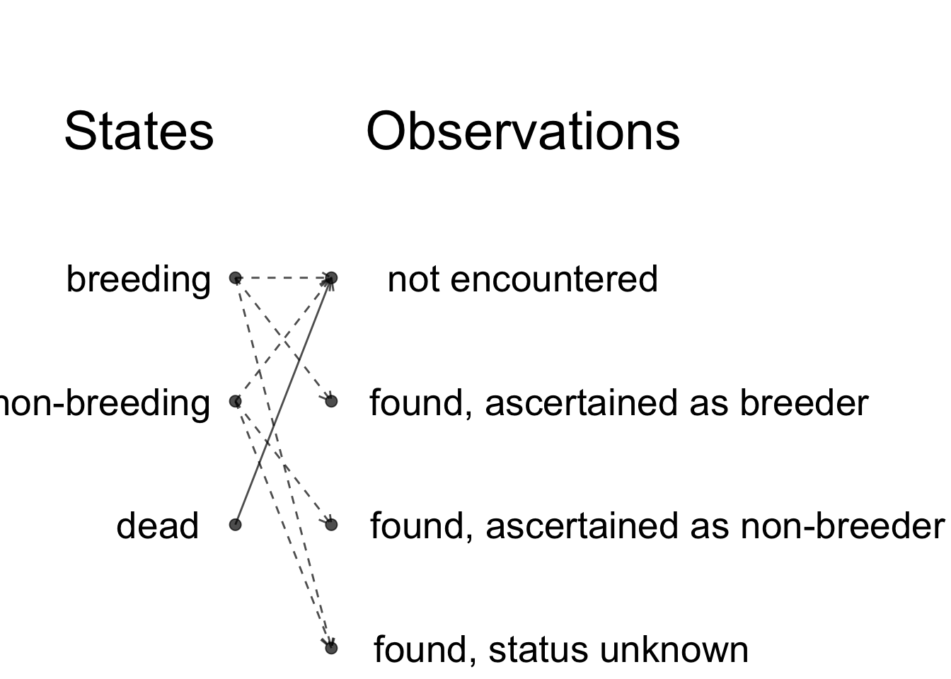
We will revisit the titis example 5.5 and try to assess life-history trade-offs while accounting for uncertainty in breeding status. We still have 3 states, which are alive and breeding, alive and non-breeding and dead. With regard to observations, a bird may be not encountered. It may also be encountered, but in contrast with our previous analysis of the titis data, we don’t know its state for sure. It may be found and ascertained (or classified) as breeder. It may be found and ascertained as non-breeder. It may be found be we are unable to determine whether it’s breeding or non-breeding.

How do the states generate the observations?

Each alive state can generate 3 observations. The only deterministic link is that between the dead state and the observation non-encountered, because if a bird is dead, it cannot be detected for sure.

Let’s specify the model. First thing we need, and it’s a big difference with the AS model, we need initial state probabilities because we cannot assign states to individuals with certainty. We write down the probability for each state at first encounter, or the vector of initial state probabilities:

\[\begin{matrix} & \\ \mathbf{\delta} = \left ( \vphantom{ \begin{matrix} 12 \end{matrix} } \right . \end{matrix} \hspace{-1.2em} \begin{matrix} z_t=B & z_t=NB & z_t=D \\ \hdashline \pi^B & 1 - \pi^{B} & 0\\ \end{matrix} \hspace{-0.2em} \begin{matrix} & \\ \left . \vphantom{ \begin{matrix} 12 \end{matrix} } \right ) \begin{matrix} \end{matrix} \end{matrix}\]

where $\pi^B$ is the probability that a newly encountered individual is a breeder, and $\pi^{NB} = 1 - \pi^B$ is the probability that a newly encountered individual is a non-breeder (the complementary probability of $\pi^B$). The probability of being dead at first encounter is 0 (a bird is alive when it is first encountered).

Now the transition matrix, this is the easy part as it doesn’t change. We have:

where $\phi^B$ is the breeder survival, $\phi_ {NB}$ that of non-breeders, $\psi^{BNB}$ is the probability for an individual breeding a year to be a non-breeder the next year, and $\psi^{NBB}$ is the probability for an non-breeder individual to breeder the next year.

Last, the observation matrix. The main difference between multisite/multistate and multievent models is here, in the observation parameters. Besides $p^B$ the detection probability of breeders and $p^{NB}$ that of non-breeders, we introduce two new parameters: $\beta^B$ is the probability to correctly assign an individual that is in state B to state B, and $\beta^{NB}$ is the probability to correctly assign an individual that is in state NB to state NB. The complementary of these $\beta$ parameters are often called false positive probabilities. We put everything in a matrix, as usual. In rows we have the states: breeding, non-breeding and dead. In columns, at the same occasion, we have the observations: non-detected, detected and ascertained B, detected and ascertained NB, and detected but state unknown:

\[\begin{matrix} & \\ \mathbf{\Omega} = \left ( \vphantom{ \begin{matrix} 12 \\ 12 \\ 12\end{matrix} } \right . \end{matrix} \hspace{-1.2em} \begin{matrix} y_t=1 & y_t=2 & y_t=3 & y_t=4\\ \hdashline 1 - p^B & p^B \beta^B & 0 & p^B (1-\beta_ B) \\ 1-p^{NB} & 0 & p^{NB} \beta^{NB} & p^{NB} (1-\beta^{NB})\\ 1 & 0 & 0 & 0 \end{matrix} \hspace{-0.2em} \begin{matrix} & \\ \left . \vphantom{ \begin{matrix} 12 \\ 12 \\ 12\end{matrix} } \right ) \begin{matrix} z_{t}=B \\ z_{t}=NB \\ z_{t}=D \end{matrix} \end{matrix}\]

For example, the probability of being detected and assigned to state B, given that you’re in state B is the product of $p^B$ the detection probability in B and $\beta^B$ the probability of correctly assigning a breeding individual to state B.

At first encounter, all individuals are captured, but you still need to assign them a state. This means that we should set $p^B = p^{NB} = 1$ and use:

\[\begin{matrix} & \\ \left ( \vphantom{ \begin{matrix} 12 \\ 12 \\ 12\end{matrix} } \right . \end{matrix} \hspace{-1.2em} \begin{matrix} y_{t = \text{first}}=1 & y_{t = \text{first}}=2 & y_{t = \text{first}}=3 & y_{t = \text{first}}=4\\ \hdashline 0 & \beta^B & 0 & (1-\beta^B)\\ 0 & 0 & \beta^{NB} & (1-\beta^{NB})\\ 1 & 0 & 0 & 0 \end{matrix} \hspace{-0.2em} \begin{matrix} & \\ \left . \vphantom{ \begin{matrix} 12 \\ 12 \\ 12\end{matrix} } \right ) \begin{matrix} z_{t = \text{first}}=B \\ z_{t = \text{first}}=NB \\ z_{t = \text{first}}=D \end{matrix} \end{matrix}\]

To implement this model in NIMBLE, we start by using comments to define the parameters, states and observations in the header of the code:

multievent <- nimbleCode({
  # -------------------------------------------------
  # Parameters:
  # phiB: survival probability state B
  # phiNB: survival probability state NB
  # psiBNB: transition probability from B to NB
  # psiNBB: transition probability from NB to B
  # pB: recapture probability B
  # pNB: recapture probability NB
  # piB prob. of being in initial state breeder
  # betaNB prob to ascertain the breeding status of an individual encountered as non-breeder
  # betaB prob to ascertain the breeding status of an individual encountered as breeder
  # -------------------------------------------------
  # States (z):
  # 1 alive B
  # 2 alive NB
  # 3 dead
  # Observations (y):
  # 1 = non-detected
  # 2 = seen and ascertained as breeder
  # 3 = seen and ascertained as non-breeder
  # 4 = not ascertained
  # -------------------------------------------------
...

Then we assign prior to all parameters to be estimated. Because we deal with probabilities, the uniform distribution between 0 and 1 will do the job:

multievent <- nimbleCode({
...
  # Priors
  phiB ~ dunif(0, 1)
  phiNB ~ dunif(0, 1)
  psiBNB ~ dunif(0, 1)
  psiNBB ~ dunif(0, 1)
  pB ~ dunif(0, 1)
  pNB ~ dunif(0, 1)
  piB ~ dunif(0, 1)
  betaNB ~ dunif(0, 1)
  betaB ~ dunif(0, 1)
...

Now we write the vector of initial state probabilities:

multievent <- nimbleCode({
...
  # vector of initial stats probs
  delta[1] <- piB # prob. of being in initial state B
  delta[2] <- 1 - piB # prob. of being in initial state NB
  delta[3] <- 0 # prob. of being in initial state dead
...

The transition matrix:

multievent <- nimbleCode({
...
  # probabilities of state z(t+1) given z(t)
  gamma[1,1] <- phiB * (1 - psiBNB)
  gamma[1,2] <- phiB * psiBNB
  gamma[1,3] <- 1 - phiB
  gamma[2,1] <- phiNB * psiNBB
  gamma[2,2] <- phiNB * (1 - psiNBB)
  gamma[2,3] <- 1 - phiNB
  gamma[3,1] <- 0
  gamma[3,2] <- 0
  gamma[3,3] <- 1
...

And the observation matrix:

multievent <- nimbleCode({
...
  # probabilities of y(t) given z(t)
  omega[1,1] <- 1 - pB             # Pr(alive B t -> non-detected t)
  omega[1,2] <- pB * betaB         # Pr(alive B t -> detected B t)
  omega[1,3] <- 0                  # Pr(alive B t -> detected NB t)
  omega[1,4] <- pB * (1 - betaB)   # Pr(alive B t -> detected U t)
  omega[2,1] <- 1 - pNB            # Pr(alive NB t -> non-detected t)
  omega[2,2] <- 0                  # Pr(alive NB t -> detected B t)
  omega[2,3] <- pNB * betaNB       # Pr(alive NB t -> detected NB t)
  omega[2,4] <- pNB * (1 - betaNB) # Pr(alive NB t -> detected U t)
  omega[3,1] <- 1                  # Pr(dead t -> non-detected t)
  omega[3,2] <- 0                  # Pr(dead t -> detected N t)
  omega[3,3] <- 0                  # Pr(dead t -> detected NB t)
  omega[3,4] <- 0                  # Pr(dead t -> detected U t)
...

The observation matrix at first encounter:

multievent <- nimbleCode({
...
  # probabilities of y(first) given z(first)
  omega.init[1,1] <- 0          # Pr(alive B t = first -> non-detected t = first)
  omega.init[1,2] <- betaB      # Pr(alive B t = first -> detected B t = first)
  omega.init[1,3] <- 0          # Pr(alive B t = first -> detected NB t = first)
  omega.init[1,4] <- 1 - betaB  # Pr(alive B t = first -> detected U t = first)
  omega.init[2,1] <- 0          # Pr(alive NB t = first -> non-detected t = first)
  omega.init[2,2] <- 0          # Pr(alive NB t = first -> detected B t = first)
  omega.init[2,3] <- betaNB     # Pr(alive NB t = first -> detected NB t = first)
  omega.init[2,4] <- 1 - betaNB # Pr(alive NB t = first -> detected U t = first)
  omega.init[3,1] <- 1          # Pr(dead t = first -> non-detected t = first)
  omega.init[3,2] <- 0          # Pr(dead t = first -> detected N t = first)
  omega.init[3,3] <- 0          # Pr(dead t = first -> detected NB t = first)
  omega.init[3,4] <- 0          # Pr(dead t = first -> detected U t = first)
...

Eventually, we get to the likelihood:

multievent <- nimbleCode({
...
  # likelihood
  for (i in 1:N){
    # latent state at first capture
    z[i,first[i]] ~ dcat(delta[1:3])
    y[i,first[i]] ~ dcat(omega.init[z[i,first[i]],1:4]) # obs at first encounter
    for (t in (first[i]+1):K){
      # z(t) given z(t-1)
      z[i,t] ~ dcat(gamma[z[i,t-1],1:3])
      # y(t) given z(t)
      y[i,t] ~ dcat(omega[z[i,t],1:4])
    }
  }
})

The only change is in the line y[i,first[i]] ~ dcat(omega.init[z[i,first[i]],1:4]) where we use the observation matrix at first encounter.

We run NIMBLE and get the following numerical summaries for the model parameters:

MCMCsummary(mcmc.multievent, round = 2)
##        mean   sd 2.5%  50% 97.5% Rhat n.eff
## betaB  0.19 0.01 0.16 0.19  0.21 1.01   332
## betaNB 0.76 0.05 0.66 0.76  0.86 1.01    65
## pB     0.56 0.03 0.51 0.56  0.62 1.06   229
## pNB    0.60 0.04 0.53 0.60  0.67 1.03   142
## phiB   0.81 0.02 0.78 0.81  0.85 1.01   312
## phiNB  0.84 0.02 0.80 0.84  0.87 1.00   354
## piB    0.71 0.03 0.66 0.71  0.76 1.02   115
## psiBNB 0.23 0.02 0.18 0.22  0.27 1.00   214
## psiNBB 0.25 0.04 0.17 0.25  0.34 1.00    95

Breeders are difficult to assign to the correct state $\beta^B$, while non-breeders are relatively well classified as non-breeders $\beta^{NB}$.

There is again no cost of current reproduction on future reproduction. We no longer detect a cost of breeding on survival.

5.7.2 Disease states

Let’s have a look to another example. We consider a system of an emerging pathogen Mycoplasma gallisepticum Edward and Kanarek and its host the house finch, Carpodacus mexicanus Müller. The pathogen causes moderate to severe eye swelling (see Figure 5.6).

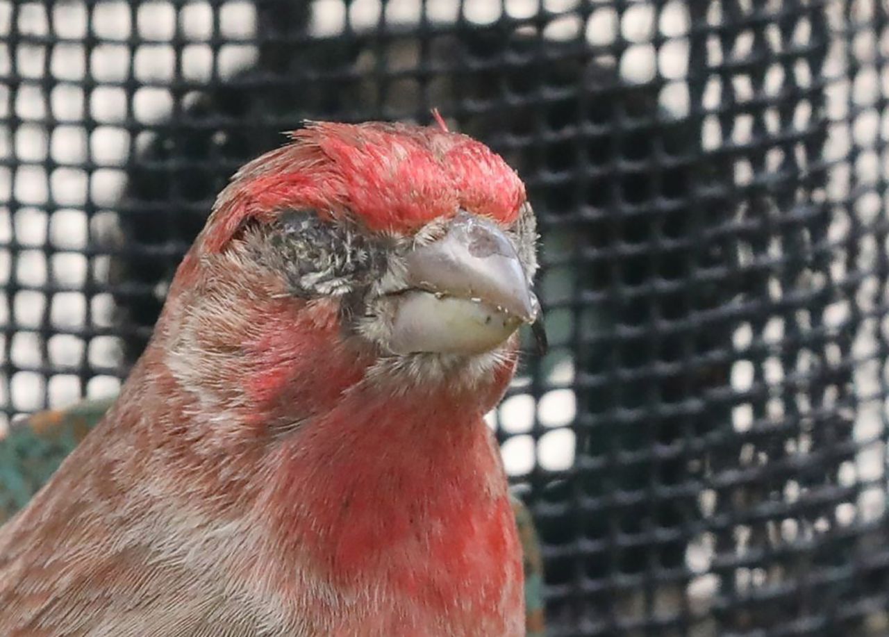
Figure 5.6: A house finch with a heavy infection caused by conjunctivitis. Credit: Jim Mondok.

Here we’re asking whether the presence of clinical signs of the pathogen influences survival. The objective of the study was also to quantify infection (moving from state healthy to state ill) and recovery (moving from state ill to state healthy) probabilities. The birds were captured via mist nets and marked with individually identifiable color bands over three years. The data were kindly provided by Paul Conn and Evan Cooch. The difficulty was that ascertaining the disease status of birds seen from distance was difficult since determining the presence of the pathogen was only possible when the bird’s eyes were clearly visible. In this context, how to study the dynamics of the disease?

First, we think of states and observations. We have:

3 states
- healthy (H)
- ill (I)
- dead (D)
4 observations
- not seen (1)
- captured healthy (2)
- captured ill (3)
- health status unknown, i.e. seen at distance (4)

How do the states generate observations?

Clearly, this is the same model as in the previous section on titis, Section 5.7.1, in which loosely speaking we replace breeder by healthy and non-breeder by ill.

The vector of initial state probabilities is:

\[\begin{matrix} & \\ \mathbf{\delta} = \left ( \vphantom{ \begin{matrix} 12 \end{matrix} } \right . \end{matrix} \hspace{-1.2em} \begin{matrix} z_t=H & z_t=I & z_t=D \\ \hdashline \pi^H & 1 - \pi^{H} & 0\\ \end{matrix} \hspace{-0.2em} \begin{matrix} & \\ \left . \vphantom{ \begin{matrix} 12 \end{matrix} } \right ) \begin{matrix} \end{matrix} \end{matrix}\]

where $\pi^H$ is the probability that a newly encountered individual is healthy, and $\pi^{I} = 1 - \pi^H$ is the probability that a newly encountered individual is ill.

The transition matrix is:

\[\begin{matrix} & \\ \mathbf{\Gamma} = \left ( \vphantom{ \begin{matrix} 12 \\ 12 \\ 12 \end{matrix} } \right . \end{matrix} \hspace{-1.2em} \begin{matrix} z_t=H & z_t=I & z_t=D \\ \hdashline \phi^H (1-\psi^{HI}) & \phi^H \psi^{HI} & 1 - \phi^H\\ \phi^{I} \psi^{IH} & \phi^{I} (1-\psi^{IH}) & 1 - \phi^{I}\\ 0 & 0 & 1 \end{matrix} \hspace{-0.2em} \begin{matrix} & \\ \left . \vphantom{ \begin{matrix} 12 \\ 12 \\ 12 \end{matrix} } \right ) \begin{matrix} z_{t-1}=H \\ z_{t-1}=I \\ z_{t-1}=D \end{matrix} \end{matrix}\]

where $\phi^H$ is the survival probability of healthy individuals, $\phi^I$ the survival probability of ill individuals, $\psi^{HI}$ the probability of getting ill (infection rate) and $\psi^{IH}$ the probability of recovering from the disease (recovery rate).

Image you’d like to model the dynamic of an incurable disease, the transition matrix would be modified by having $\psi^{IH} = 0$, and once a bird gets ill, it remains ill $\psi^{II} = 1 - \psi^{IH} = 1$. Therefore we would have:

\[\begin{matrix} & \\ \mathbf{\Gamma} = \left ( \vphantom{ \begin{matrix} 12 \\ 12 \\ 12 \end{matrix} } \right . \end{matrix} \hspace{-1.2em} \begin{matrix} z_t=H & z_t=I & z_t=D \\ \hdashline \phi^H (1-\psi^{HI}) & \phi^H \psi^{HI} & 1 - \phi^H\\ 0 & \phi^{I} & 1 - \phi^{I}\\ 0 & 0 & 1 \end{matrix} \hspace{-0.2em} \begin{matrix} & \\ \left . \vphantom{ \begin{matrix} 12 \\ 12 \\ 12 \end{matrix} } \right ) \begin{matrix} z_{t-1}=H \\ z_{t-1}=I \\ z_{t-1}=D \end{matrix} \end{matrix}\]

For analysing the house finch data, we allow recovering from the disease. The observation matrix is:

\[\begin{matrix} & \\ \mathbf{\Omega} = \left ( \vphantom{ \begin{matrix} 12 \\ 12 \\ 12\end{matrix} } \right . \end{matrix} \hspace{-1.2em} \begin{matrix} y_t=0 & y_t=1 & y_t=2 & y_t=3\\ \hdashline 1-p^H & p^H \beta^H & 0 & p^H (1-\beta^H)\\ 1-p^I & 0 & p^{I} \beta^{I} & p^{I} (1-\beta^{I})\\ 1 & 0 & 0 & 0 \end{matrix} \hspace{-0.2em} \begin{matrix} & \\ \left . \vphantom{ \begin{matrix} 12 \\ 12 \\ 12\end{matrix} } \right ) \begin{matrix} z_{t}=H \\ z_{t}=I \\ z_{t}=D \end{matrix} \end{matrix}\]

where $\beta^H$ is the probability to assign a healthy individual to state H, and $\beta^{I}$ is the probability to assign a sick individual to state I. $p^H$ is the detection probability of healthy individuals, $p^I$ that of sick individuals.

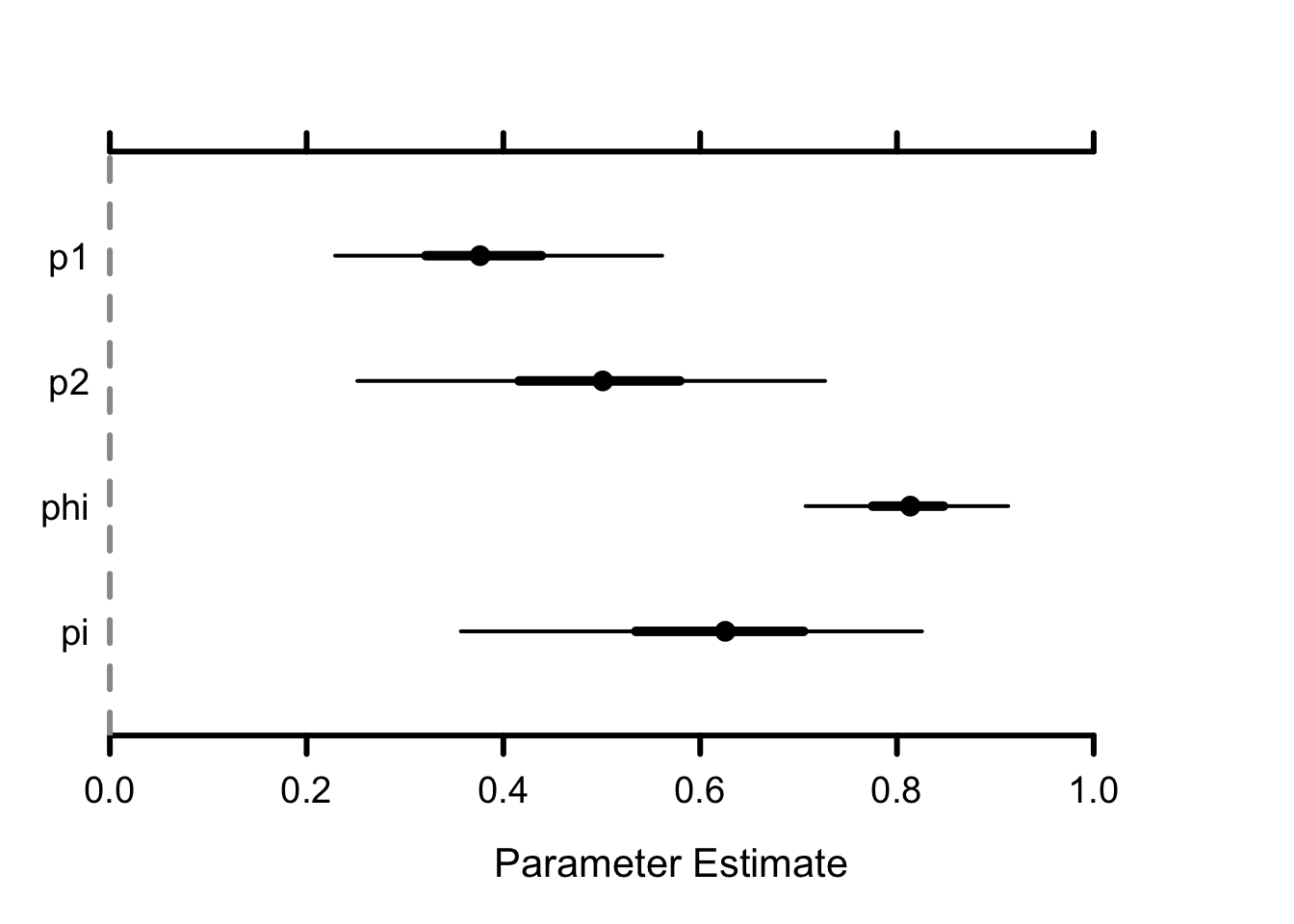
Using the code we developped for the titis example, we get the following results on the finches by running NIMBLE:

##       mean   sd 2.5%  50% 97.5% Rhat n.eff
## betaH 0.99 0.01 0.97 0.99  1.00 1.01  1421
## betaI 0.05 0.01 0.03 0.05  0.08 1.00  6477
## pH    0.17 0.02 0.13 0.17  0.22 1.01   331
## pI    0.58 0.10 0.41 0.57  0.80 1.04   220
## phiH  0.88 0.02 0.84 0.88  0.92 1.01   360
## phiI  0.99 0.01 0.96 0.99  1.00 1.00  1004
## pi    0.96 0.01 0.93 0.96  0.98 1.00  4190
## psiHI 0.22 0.04 0.16 0.22  0.32 1.02   311
## psiIH 0.46 0.08 0.32 0.45  0.63 1.02   392

Healthy individuals are correctly assigned ($\beta^H$ is almost 1), while infected individuals are difficult to ascertain ($\beta^I$ is around 0.05). Unexpectedly, ill birds have a better survival than healthy individuals (compare $\phi^I$ and $\phi^H$). Infection rate ($\psi^{HI}$) is 22%, recovery rate is 46% ($\psi^{IH}$).

5.8 Summary

The AS model is a HMM that extends the CJS model by allowing the estimation of movements between sites (e.g. geographical locations) or transitions between states (e.g. breeding status). This flexibility allows addressing all sorts of questions in ecology and evolution.
Covariates can be considered, and appropriate priors or link functions need to be used when there are more than 2 sites or 2 alive states.
Model comparison can be achieved with the WAIC and the goodness of fit of the AS model to capture-recapture data can be assessed with classical procedures or posterior predictive checks.
Importantly, the HMM framework allows to account for uncertainty when assigning states to individuals.
The models covered in this chapter haven been called multistratum/strata models, multisite models (section 5.2), multistate models (section 5.5) and multievent models (section 5.7). These models are all HMMs.

5.9 Suggested reading

The AS model was introduced in Arnason (1972), Arnason (1973) and Schwarz, Schweigert, and Arnason (1993). Very soon clever folks realized that sites could be replaced by states as in Nichols et al. (1992) and Nichols et al. (1994). For a review of models with sites and states, see Lebreton et al. (2009).
The geese data were analyzed in Hestbeck, Nichols, and Malecki (1991) and Brownie et al. (1993), and the titis data in Scofield, Fletcher, and Robertson (2001). The house finches data were analyzed in Faustino et al. (2004) and Conn and Cooch (2009) (see also Cooch et al. (2012)). Check out Santoro et al. (2014), Marescot et al. (2018) and Ollivier et al. (2023) for other examples in disease ecology.
Section 5.6 on local minima was inspired by chapter 10 of Cooch and White (2017).
Classical goodness of fit tests are reviewed in Pradel, Gimenez, and Lebreton (2005). See also Pradel, Wintrebert, and Gimenez (2003) for tests specifically designed for multisite/multistate models.
Models with uncertainty were introduced in Pradel (2005). Dupuis (1995) had a similar idea for the AS model. For a review, see Gimenez et al. (2012).

4 Alive and dead

Introduction