1 Bayesian statistics & MCMC
1.1 Introduction
In this first chapter, you will learn what the Bayesian theory is, and how you may use it with a simple example. You will also see how to implement simulation algorithms to implement the Bayesian method for more complex analyses. This is not an exhaustive treatment of Bayesian statistics, but you should get what you need to navigate through the rest of the book.
1.2 Bayes’ theorem
Let’s not wait any longer and jump into it. Bayesian statistics relies on the Bayes’ theorem (or law, or rule, whatever you prefer) named after Reverend Thomas Bayes (Figure 1.1). This theorem was published in 1763 two years after Bayes’ death thanks to his friend’s efforts Richard Price, and was independently discovered by Pierre-Simon Laplace (McGrayne 2011).

Figure 1.1: Cartoon of Thomas Bayes with Bayes’ theorem in background. Source: James Kulich at https://www.elmhurst.edu/blog/thomas-bayes/
As we will see in a minute, Bayes’ theorem is all about conditional probabilities, which are somehow tricky to understand. Conditional probability of outcome or event A given event B, which we denote \(\Pr(A \mid B)\), is the probability that A occurs, revised by considering the additional information that event B has occurred. For example, a friend of yours rolls a fair dice and asks you the probability that the outcome was a six (event A). Your answer is 1/6 because each side of the dice is equally likely to come up. Now imagine that you’re told the number rolled was even (event B) before you answer your friend’s question. Because there are only three even numbers, one of which is six, you may revise your answer for the probability that a six was rolled from 1/6 to \(\Pr(A \mid B) = 1/3\). The order in which A and B appear is important, make sure you do not confuse \(\Pr(A \mid B)\) and \(\Pr(B \mid A)\).
Bayes’ theorem gives you \(\Pr(A \mid B)\) using marginal probabilities \(\Pr(A)\) and \(\Pr(B)\) and \(\Pr(B \mid A)\):
\[\Pr(A \mid B) = \displaystyle{\frac{ \Pr(B \mid A) \; \Pr(A)}{\Pr(B)}}.\]
We talk about a marginal probability when we are interested in the probability of an event “on its own”, without any particular condition. For example, \(\Pr(A)\) or \(\Pr(B)\) are the overall chances of \(A\) or \(B\), without taking anything else into account. It is called marginal because, if you built a table with all possible combinations (for instance, dice outcomes classified as even/odd and as “six/not six”), then \(\Pr(A)\) and \(\Pr(B)\) are obtained by adding up the entries of a row or a column, that is, what you read in the margins of the table.
Originally, Bayes’ theorem was seen as a way to infer an unkown cause A of a particular effect B, knowing the probability of effect B given cause A. Think for example of a situation where a medical diagnosis is needed, with A an unknown disease and B symptoms, the doctor knows Pr(symptoms|disease) and wants to derive Pr(disease|symptoms). This way of reversing \(\Pr(B \mid A)\) into \(\Pr(A \mid B)\) explains why Bayesian thinking used to be referred to as ‘inverse probability’.
I don’t know about you, but I need to think twice for not messing the letters around.
I find it easier to remember Bayes’ theorem written like this:
\[\Pr(\text{hypothesis} \mid \text{data}) = \frac{ \Pr(\text{data} \mid \text{hypothesis}) \; \Pr(\text{hypothesis})}{\Pr(\text{data})}\] The hypothesis is a working assumption about which you want to learn using data. In capture–recapture analyses, the hypothesis might be a parameter like detection probability, or regression parameters in a relationship between survival probability and a covariate (see Chapter 4). Bayes’ theorem tells us how to obtain the probability of a hypothesis given the data we have.
This is great because think about it, this is exactly what the scientific method is! We’d like to know how plausible some hypothesis is based on some data we collected, and possibly compare several hypotheses among them. In that respect, the Bayesian reasoning matches the scientific reasoning, which probably explains why the Bayesian framework is so natural for doing and understanding statistics.
You might ask then, why is Bayesian statistics not the default in statistics? Until recently, there were practical problems to implement Bayes’ theorem. Recent advances in computational power coupled with the development of new algorithms have led to a great increase in the application of Bayesian methods within the last three decades.
1.3 What is the Bayesian approach?
Typical statistical problems involve estimating a parameter (or several parameters) \(\theta\) with available data. To do so, you might be more used to the frequentist rather than the Bayesian method. The frequentist approach, and in particular maximum likelihood estimation (MLE), assumes that the parameters are fixed, and have unknown values to be estimated. Therefore classical estimates are generally point estimates of the parameters of interest. In contrast, the Bayesian approach assumes that the parameters are not fixed, and have some unknown distribution. A probability distribution is a mathematical expression that gives the probability for a random variable to take particular values. It may be either discrete (e.g., the Bernoulli, Binomial or Poisson distribution) or continuous (e.g., the Gaussian distribution also known as the normal distribution).
The Bayesian approach is based upon the idea that you, as an experimenter, begin with some prior beliefs about the system. Then you collect data and update your prior beliefs on the basis of observations. These observations might arise from field work, lab work or from expertise of your esteemed colleagues. This updating process is based upon Bayes’ theorem. Loosely, let’s say \(A = \theta\) and \(B = \text{data}\), then Bayes’ theorem gives you a way to estimate parameter \(\theta\) given the data you have:
\[{\color{red}{\Pr(\theta \mid \text{data})}} = \frac{\color{blue}{\Pr(\text{data} \mid \theta)} \times \color{green}{\Pr(\theta)}}{\color{orange}{\Pr(\text{data})}}.\] Let’s spend some time going through each quantity in this formula.
On the left-hand side is \(\color{red}{\Pr(\theta \mid \text{data})}\) the \(\color{red}{\text{posterior distribution}}\). It represents what you know after having seen the data. This is the basis for inference and clearly what you’re after, a distribution, possibly multivariate if you have more than one parameter.
On the right-hand side, there is \(\color{blue}{\Pr(\text{data} \mid \theta)}\) the \(\color{blue}{\text{likelihood}}\). This quantity is the same as in the MLE approach. Yes, the Bayesian and frequentist approaches have the same likelihood at their core, which mostly explains why results often do not differ much. The likelihood captures the information you have in your data, given a model parameterized with \(\theta\).
Then we have \(\color{green}{\Pr(\theta)}\) the \(\color{green}{\text{prior distribution}}\). This quantity represents what you know before seeing the data. This is the source of much discussion about the Bayesian approach. It may be vague if you don’t know anything about \(\theta\). Usually however, you never start from scratch, and you’d like your prior to reflect the information you have (see Section 4.9 for how to accomplish that).
Last, we have \(\color{orange}{\Pr(\text{data})}\) which is sometimes called the average likelihood because it is obtained by integrating the likelihood with respect to the prior \(\color{orange}{\Pr(\text{data}) = \int{\Pr(\text{data} \mid \theta)\Pr(\theta) d\theta}}\) so that the posterior is standardized, that is it integrates to one for the posterior to be a distribution. The average likelihood is an integral with dimension the number of parameters \(\theta\) you need to estimate. This quantity is difficult, if not impossible, to calculate in general. This is one of the reasons why the Bayesian method wasn’t used until recently, and why we need algorithms to estimate posterior distributions as I illustrate in the next section.
1.4 Approximating posteriors via numerical integration
Let’s take an example to illustrate Bayes’ theorem. Say we capture, mark and release \(n = 57\) animals at the beginning of a winter, out of which we recapture \(y = 19\) animals alive (we used a similar example in King et al. 2009). We’d like to estimate winter survival \(\theta\). The data are:
y <- 19 # nb of success
n <- 57 # nb of attempts
We build our model first. Assuming all animals are independent of each other and have the same survival probability, then \(y\) the number of alive animals at the end of the winter is a binomial distribution with \(n\) trials and \(\theta\) the probability of success:
\[\begin{align*} y &\sim \text{Binomial}(n, \theta) &\text{[likelihood]} \end{align*}\]
Note that I follow McElreath (2020) and use labels on the right to help remember what each line is about. This likelihood can be visualised in R:
grid <- seq(0, 1, 0.01) # grid of values for survival
likelihood <- dbinom(y, n, grid) # compute binomial likelihood
df <- data.frame(survival = grid, likelihood = likelihood)
df %>%
  ggplot() +
  aes(x = survival, y = likelihood) +
  geom_line(linewidth = 1.5)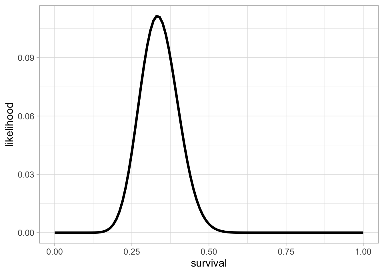
This is the binomial likelihood with \(n = 57\) released animals and \(y = 19\) survivors after winter. The value of survival (on the x-axis) that corresponds to the maximum of the likelihood function (on the y-axis) is the MLE, or the proportion of success in this example, close to 0.33.
Besides the likelihood, priors are another component of the model in the Bayesian approach. For a parameter that is a probability, the one thing we know is that the prior should be a continuous random variable that lies between 0 and 1. To reflect that, we often go for the uniform distribution \(U(0,1)\) to imply vague priors. Here vague means that survival has, before we see the data, the same probability of falling between 0.1 and 0.2 and between 0.8 and 0.9, for example.
\[\begin{align*} \theta &\sim \text{Uniform}(0, 1) &\text{[prior for }\theta \text{]} \end{align*}\]
Now we apply Bayes’ theorem. We write a R function that computes the product of the likelihood times the prior, or the numerator in Bayes’ theorem: \(\Pr(\text{data} \mid \theta) \times \Pr(\theta)\)
We write another function that calculates the denominator, the average likelihood: \(\Pr(\text{data}) = \int{\Pr(\text{data} \mid \theta) \Pr(\theta) d\theta}\)
denominator <- integrate(numerator,0,1)$valueWe use the R function integrate to calculate the integral in the denominator, which implements quadrature techniques to divide in little squares the area underneath the curve delimited by the function to integrate (here the numerator), and count them.
Then we get a numerical approximation of the posterior of winter survival by applying Bayes’ theorem:
grid <- seq(0, 1, 0.01) # grid of values for theta
numerical_posterior <- data.frame(survival = grid,
  posterior = numerator(grid)/denominator) # Bayes' theorem
numerical_posterior %>%
  ggplot() +
  aes(x = survival, y = posterior) +
  geom_line(linewidth = 1.5)
How good is our numerical approximation of survival posterior distribution? Ideally, we would want to compare the approximation to the true posterior distribution. Although a closed-form expression for the posterior distribution is in general intractable, when you combine a binomial likelihood together with a beta distribution as a prior, then the posterior distribution is also a beta distribution, which makes it amenable to all sorts of exact calculations. We say that the beta distribution is the conjugate prior distribution for the binomial distribution. The beta distribution is continuous between 0 and 1, and extends the uniform distribution to situations where not all outcomes are equally likely. It has two parameters \(a\) and \(b\) that control its shape (Figure 1.2).
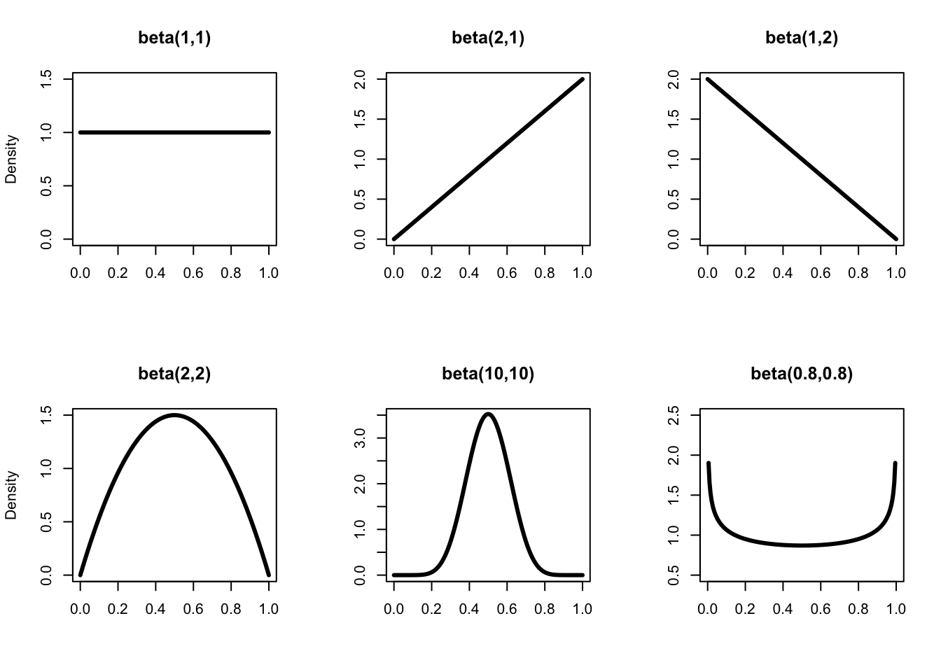
Figure 1.2: The distribution beta(\(a\),\(b\)) for different values of \(a\) and \(b\). Note that for \(a = b = 1\), we get the uniform distribution between 0 and 1 in the top left panel. When \(a\) and \(b\) are equal, the distribution is symmetric, and the bigger \(a\) and \(b\), the more peaked the distribution around the mean (the smaller the variance). The expectation (or mean) of a beta(\(a\),\(b\)) is \(\displaystyle{\frac{a}{a + b}}\).
If the likelihood of the data \(y\) is binomial with \(n\) trials and probability of success \(\theta\), and the prior is a beta distribution with parameters \(a\) and \(b\), then the posterior is a beta distribution with parameters \(a + y\) and \(b + n - y\). In our example, we have \(n = 57\) trials and \(y = 19\) animals that survived and a uniform prior between 0 and 1 or a beta distribution with parameters \(a = b = 1\), therefore survival has a beta posterior distribution with parameters 20 and 39. Let’s superimpose the exact posterior and the numerical approximation:
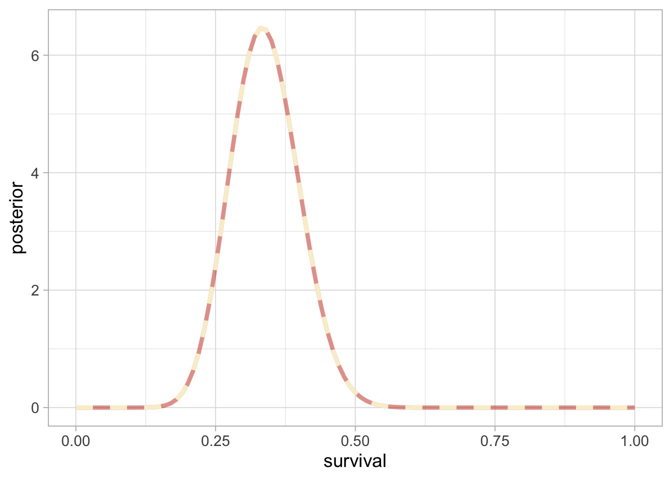
Clearly, the exact (black or brick-red in the online version) vs. numerical approximation (grey or cream in the online version) of winter survival posterior distribution are indistinguishable, suggesting that the numerical approximation is more than fine.
In our example, we have a single parameter to estimate, winter survival. This means dealing with a one-dimensional integral in the denominator which is pretty easy with quadrature techniques and the R function integrate(). Now what if we had multiple parameters? For example, imagine you’d like to fit a capture-recapture model with detection probability \(p\) and regression parameters \(\alpha\) and \(\beta\) for the intercept and slope of a relationship between survival probability and a covariate, then Bayes’ theorem gives you the posterior distribution of all three parameters together:
\[ \Pr(\alpha, \beta, p \mid \text{data}) = \frac{ \Pr(\text{data} \mid \alpha, \beta, p) \times \Pr(\alpha, \beta, p)}{\iiint \, \Pr(\text{data} \mid \alpha, \beta, p) \Pr(\alpha, \beta, p) d\alpha d\beta dp} \] There are two computational challenges with this formula. First, do we really wish to calculate a three-dimensional integral? The answer is no, one-dimensional and two-dimensional integrals are so much further we can go with standard methods. Second, we’re more interested in a posterior distribution for each parameter separately than the joint posterior distribution. The so-called marginal distribution of \(p\) for example is obtained by integrating over all the other parameters – a two-dimensional integral in this example. Now imagine with tens or hundreds of parameters to estimate, these integrals become highly multi-dimensional and simply intractable. In the next section, I introduce powerful simulation methods to circumvent this issue.
1.5 Markov chain Monte Carlo (MCMC)
In the early 1990s, statisticians rediscovered work from the 1950’s in physics. In a famous paper that would lay the fundations of modern Bayesian statistics (Figure 1.3), the authors use simulations to approximate posterior distributions with some precision by drawing large samples. This is a neat trick to avoid explicit calculation of the multi-dimensional integrals we struggle with when using Bayes’ theorem.
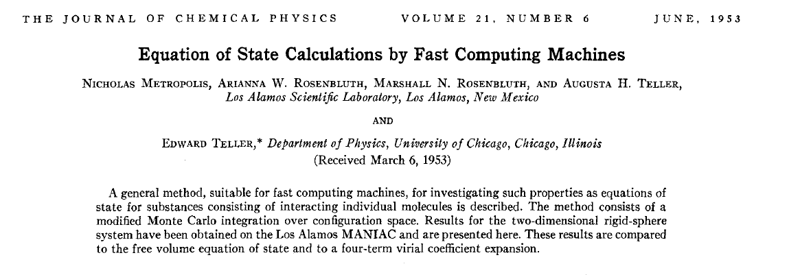
Figure 1.3: MCMC article cover. Source: The Journal of Chemical Physics – https://aip.scitation.org/doi/10.1063/1.1699114
These simulation algorithms are called Markov chain Monte Carlo (MCMC), and they definitely gave a boost to Bayesian statistics. There are two parts in MCMC, Markov chain and Monte Carlo, let’s try and make sense of these terms.
1.5.1 Monte Carlo integration
What does Monte Carlo stand for? Monte Carlo integration is a simulation technique to calculate integrals of any function \(f\) of random variable \(X\) with distribution \(\Pr(X)\) say \(\int f(X) \Pr(X)dX\). You draw values \(X_1,\ldots,X_k\) from \(\Pr(X)\) the distribution of \(X\), apply function \(f\) to these values, then calculate the mean of these new values \(\displaystyle{\frac{1}{k}}\sum_{i=1}^k{f(X_i)}\) to approximate the integral. How is Monte Carlo integration used in a Bayesian context? The posterior distribution contains all the information we need about the parameter to be estimated. When dealing with many parameters however, you may want to summarise posterior results by calculating numerical summaries. The simplest numerical summary is the mean of the posterior distribution, \(E(\theta) = \int \theta \Pr(\theta|\text{data})\), where \(X\) is \(\theta\) now and \(f\) is the identity function. Posterior mean can be calculated with Monte Carlo integration:
# draw 1000 values from posterior survival beta(20,39)
sample_from_posterior <- rbeta(1000, 20, 39)
# compute mean with Monte Carlo integration
mean(sample_from_posterior)
## [1] 0.3397
You may check that the mean we have just calculated matches closely the expectation of a beta distribution:
20/(20+39) # expectation of beta(20,39)
## [1] 0.339
Another useful numerical summary is the credible interval within which our parameter falls with some probability, usually 0.95 hence a 95\(\%\) credible interval. Finding the bounds of a credible interval requires calculating quantiles, which in turn involves integrals and the use of Monte Carlo integration. A 95\(\%\) credible interval for winter survival can be obtained in R with:
1.5.2 Markov chains
What is a Markov chain? A Markov chain is a random sequence of numbers, in which each number depends only on the previous number. An example is the weather in my home town in Southern France, Montpellier, in which a sunny day is most likely to be followed by another sunny day, say with probability 0.8, and a rainy day is rarely followed by another rainy day, say with probability 0.1. The dynamic of this Markov chain is captured by the transition matrix \(\Gamma\): \[ \begin{matrix} & \\ \Gamma = \left ( \vphantom{ \begin{matrix} 12 \\ 12 \end{matrix} } \right . \end{matrix} \hspace{-1.2em} \begin{matrix} \text{sunny tomorrow} & \text{rainy tomorrow} \\[0.3em] 0.8 & 0.2 \\ 0.9 & 0.1 \\ \end{matrix} \hspace{-0.2em} \begin{matrix} & \\ \left . \vphantom{ \begin{matrix} 12 \\ 12 \end{matrix} } \right ) \begin{matrix} \text{sunny today} \\ \text{rainy today} \end{matrix} \end{matrix} \]
In rows the weather today, and in columns the weather tomorrow. The cells give the probability of a sunny or rainy day tomorrow, given the day is sunny or rainy today. Under certain conditions, a Markov chain will converge to a unique stationary distribution. In our weather example, let’s run the Markov chain for 20 steps:
# transition matrix
weather <- matrix(c(0.8, 0.2, 0.9, 0.1), nrow = 2, byrow = T)
steps <- 20
for (i in 1:steps){
  weather <- weather %*% weather # matrix multiplication
}
round(weather, 2) # matrix product after 20 steps
##      [,1] [,2]
## [1,] 0.82 0.18
## [2,] 0.82 0.18
Each row of the transition matrix converges to the same distribution \((0.82, 0.18)\) as the number of steps increases. Convergence happens no matter which state you start in, and you always have probability 0.82 of the day being sunny and 0.18 of the day being rainy.
Back to MCMC, the core idea is that you can build a Markov chain with a given stationary distribution set to be the desired posterior distribution.
Putting Monte Carlo and Markov chains together, MCMC allows us to generate a sample of values (Markov chain) whose distribution converges to the posterior distribution, and we can use this sample of values to calculate any posterior summaries (Monte Carlo), such as posterior means and credible intervals.
1.5.3 Metropolis algorithm
There are several ways of constructing Markov chains for Bayesian inference. You might have heard about the Metropolis-Hastings or the Gibbs sampler. Have a look to https://chi-feng.github.io/mcmc-demo/ for an interactive gallery of MCMC algorithms. Here I illustrate the Metropolis algorithm and how to implement it in practice.
Let’s go back to our example on animal survival estimation. We illustrate sampling from survival posterior distribution. We write functions for likelihood, prior and posterior:
# 19 recaptured alive out of 57 captured, marked and released
survived <- 19
released <- 57

# binomial log-likelihood function
loglikelihood <- function(x, p){
  dbinom(x = x, size = released, prob = p, log = TRUE)
}

# uniform prior density
logprior <- function(p){
  dunif(x = p, min = 0, max = 1, log = TRUE)
}

# posterior density function (log scale)
posterior <- function(x, p){
  loglikelihood(x, p) + logprior(p) # - log(Pr(data))
}
The Metropolis algorithm works as follows:
We pick a value of the parameter to be estimated. This is where we start our Markov chain – this is a starting value, or a starting location.
To decide where to go next, we propose to move away from the current value of the parameter – this is a candidate value. To do so, we add to the current value some random value from e.g. a normal distribution with some variance – this is a proposal distribution. The Metropolis algorithm is a particular case of the Metropolis-Hastings algorithm with symmetric proposals.
We compute the ratio of the probabilities at the candidate and current locations \(R=\displaystyle{\frac{{\Pr(\text{candidate}|\text{data})}}{{\Pr(\text{current}|\text{data})}}}\). This is where the magic of MCMC happens, in that \(\Pr(\text{data})\), the denominator in the Bayes’ theorem, appears in both the numerator and the denominator in \(R\) therefore cancels out and does not need to be calculated.
If the posterior at the candidate location \(\Pr(\text{candidate}|\text{data})\) is higher than at the current location \(\Pr(\text{current}|\text{data})\), in other words when the candidate value is more plausible than the current value, we definitely accept the candidate value. If not, then we accept the candidate value with probability \(R\) and reject with probability \(1-R\). For example, if the candidate value is ten times less plausible than the current value, then we accept with probability 0.1 and reject with probability 0.9. How does it work in practice? We use a continuous spinner that lands somewhere between 0 and 1 – call the random spin \(X\). If \(X\) is smaller than \(R\), we move to the candidate location, otherwise we remain at the current location. We do not want to accept or reject too often. In practice, the Metropolis algorithm should have an acceptance probability between 0.2 and 0.4, which can be achieved by tuning the variance of the normal proposal distribution.
We repeat 2-4 a number of times – or steps.
Enough of the theory, let’s implement the Metropolis algorithm in R. Let’s start by setting the scene:
steps <- 100 # number of steps
theta.post <- rep(NA, steps) # vector to store samples
accept <- rep(NA, steps) # keep track of accept/reject
set.seed(1234) # for reproducibility
Now follow the 5 steps we’ve just described. First, we pick a starting value, and store it (step 1):
inits <- 0.5
theta.post[1] <- inits
accept[1] <- 1
Then, we need a function to propose a candidate value:
# by default, standard deviation of the proposal distribution is 1
move <- function(x, away = 1){
  # apply logit transform (-infinity,+infinity)
  logitx <- log(x / (1 - x))
  # add a value taken from N(0,sd=away) to current value
  logit_candidate <- logitx + rnorm(1, 0, away)
  # back-transform (0,1)
  candidate <- plogis(logit_candidate)
  return(candidate)
}
We add a value taken from a normal distribution with mean zero and standard deviation we call away. We work on the logit scale to make sure the candidate value for survival lies between 0 and 1.
Now we’re ready for steps 2, 3 and 4. We write a loop to take care of step 5. We start at initial value 0.5 and run the algorithm for 100 steps or iterations:
for (t in 2:steps){ # repeat steps 2-4 (step 5)

  # propose candidate value for survival (step 2)
  theta_star <- move(theta.post[t-1])

  # calculate ratio R (step 3)
  pstar <- posterior(survived, p = theta_star)
  pprev <- posterior(survived, p = theta.post[t-1])
  logR <- pstar - pprev # likelihood and prior are on the log scale
  R <- exp(logR)

  # accept candidate value or keep current value (step 4)
  X <- runif(1, 0, 1) # spin continuous spinner
  if (X < R){
    theta.post[t] <- theta_star # accept candidate value
    accept[t] <- 1 # accept
  }
  else{
    theta.post[t] <- theta.post[t-1] # keep current value
    accept[t] <- 0 # reject
  }
}
We get the following values:
head(theta.post) # first values
## [1] 0.5000 0.2302 0.2906 0.2906 0.2980 0.2980
tail(theta.post) # last values
## [1] 0.2622 0.2622 0.2622 0.3727 0.3232 0.3862
Visually, you may look at the chain:
df <- data.frame(x = 1:steps, y = theta.post)
df %>%
  ggplot() +
  geom_line(aes(x = x, y = y),
            size = 1.5,
            color = wesanderson::wes_palettes$Zissou1[1]) +
  labs(x = "iterations", y = "samples") +
  ylim(0.1, 0.6)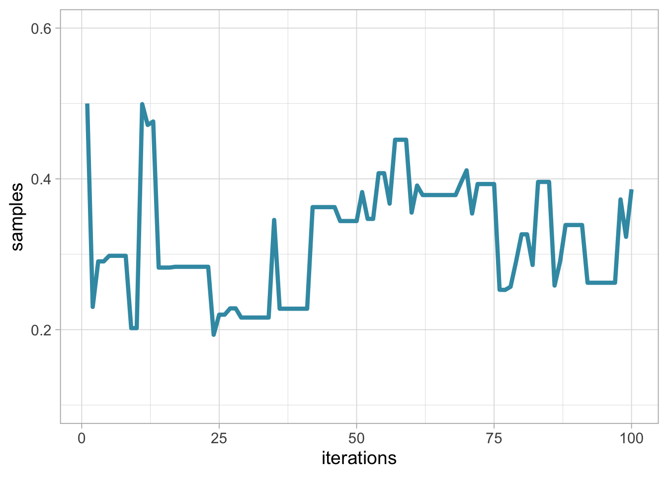
In this visualisation, remember that our Markov chain starts at value 0.5. The steps or iterations are on the x-axis, and samples on the y-axis. This graphical representation is called a trace plot.
The acceptance probability is the average number of times we accepted a candidate value, which is 0.44 and almost satisfying.
To make our life easier and avoid repeating the same lines of code again and again, let’s make a function out of the code we have written so far:
metropolis <- function(steps = 100, inits = 0.5, away = 1){

  # pre-alloc memory
  theta.post <- rep(NA, steps)

  # start
  theta.post[1] <- inits

  for (t in 2:steps){

    # propose candidate value for prob of success
    theta_star <- move(theta.post[t-1], away = away)

    # calculate ratio R
    pstar <- posterior(survived, p = theta_star)
    pprev <- posterior(survived, p = theta.post[t-1])
    logR <- pstar - pprev
    R <- exp(logR)

    # accept candidate value or keep current value (step 4)
    X <- runif(1, 0, 1) # spin continuous spinner
    if (X < R){
      theta.post[t] <- theta_star
    }
    else{
      theta.post[t] <- theta.post[t-1]
    }
  }
  theta.post
}
Can we run another chain and start at initial value 0.2 this time? Yes, just go through the same algorithm again, and visualise the results with trace plot of survival for two chains starting at 0.2 (grey, or yellow in the online version) and 0.5 (black, or blue in the online version) run for 100 steps:
theta.post2 <- metropolis(steps = 100, inits = 0.2)
df2 <- data.frame(x = 1:steps, y = theta.post2)

if (params$bw) {
  ggplot() +
  geom_line(data = df,
            aes(x = x, y = y),
            size = 1.5,
            color = 'black') +
  geom_line(data = df2,
            aes(x = x, y = y),
            size = 1.5,
            color = 'grey') +
  labs(x = "iterations", y = "values from posterior distribution") +
  ylim(0.1, 0.6)

} else {
  ggplot() +
  geom_line(data = df,
            aes(x = x, y = y),
            size = 1.5,
            color = wesanderson::wes_palettes$Zissou1[1]) +
  geom_line(data = df2,
            aes(x = x, y = y),
            size = 1.5,
            color = wesanderson::wes_palettes$Zissou1[3]) +
  labs(x = "iterations", y = "values from posterior distribution") +
  ylim(0.1, 0.6)
}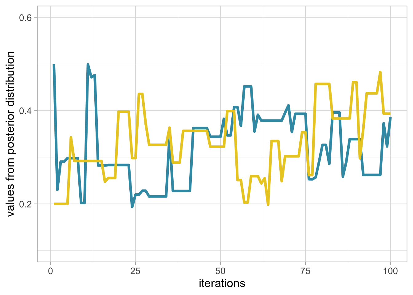
Notice that we do not get the exact same results because the algorithm is stochastic. The question is to know whether we have reached the stationary distribution. Let’s increase the number of steps, start at 0.5 and run a chain with 5000 iterations:
steps <- 5000
set.seed(1234)
theta.post <- metropolis(steps = steps, inits = 0.5)
df <- data.frame(x = 1:steps, y = theta.post)
df %>%
  ggplot() +
  geom_line(aes(x = x, y = y),
            size = 1,
            color = wesanderson::wes_palettes$Zissou1[1]) +
  labs(x = "iterations", y = "values from posterior distribution") +
  ylim(0.1, 0.6) +
  geom_hline(aes(yintercept = mean(theta.post),
                 linetype = "posterior mean")) +
scale_linetype_manual(name = "", values = c(2,2)) 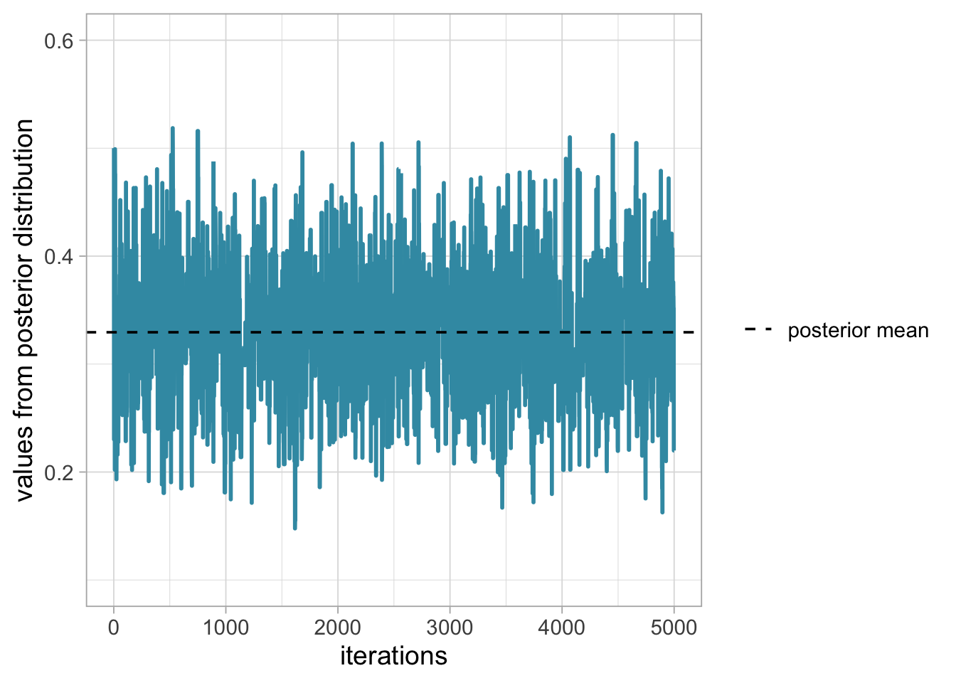
This is what we’re after, a trace plot that looks like a beautiful lawn, see Section 1.6.
Once the stationary distribution is reached, you may regard the realisations of the Markov chain as a sample from the posterior distribution, and obtain numerical summaries. In the next section, we consider several important implementation issues.
1.6 Assessing convergence
When implementing MCMC, we need to determine how long it takes for our Markov chain to converge to the target distribution, and the number of iterations we need after achieving convergence to get reasonable Monte Carlo estimates of numerical summaries (posterior means and credible intervals).
1.6.1 Burn-in
In practice, we discard observations from the start of the Markov chain and just use observations from the chain once it has converged. The initial observations that we discard are usually referred to as the burn-in.
The simplest method to determine the length of the burn-in period is to look at trace plots. Going back to our example, let’s have a look to a trace plot of a chain that starts at value 0.99.
# set up the scene
steps <- 1000
theta.post <- metropolis(steps = steps, inits = 0.99)
df <- data.frame(x = 1:steps, y = theta.post)
df %>%
  ggplot() +
  geom_line(aes(x = x, y = y),
            size = 1.2,
            color = wesanderson::wes_palettes$Zissou1[1]) +
  labs(x = "iterations", y = "survival") +
  theme_light(base_size = 14) +
  annotate("rect",
           xmin = 0,
           xmax = 100,
           ymin = 0.1,
           ymax = 1,
           alpha = .3) +
  scale_y_continuous(expand = c(0,0))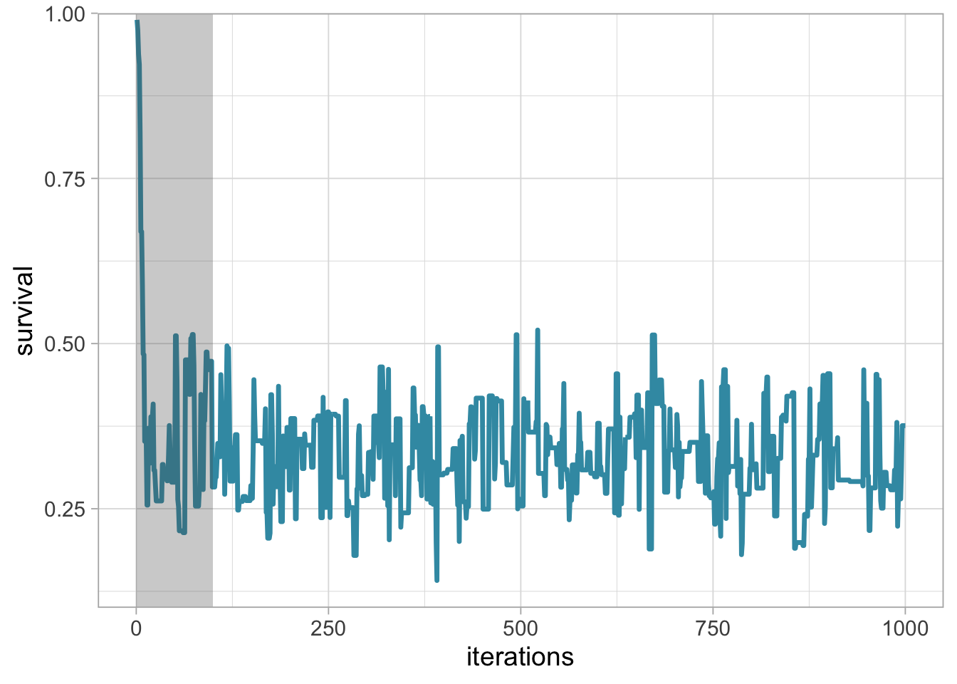
The chain starts at value 0.99 and rapidly stabilises, with values bouncing back and forth around 0.3 from the 100th iteration onwards. You may choose the shaded area as the burn-in, and discard the first 100th values.
We see from the trace plot below that we need at least 100 iterations to achieve convergence toward an average survival around 0.3. It is always better to be conservative when specifying the length of the burn-in period, and in this example, we would use 250 or even 500 iterations as a burn-in. The length of the burn-in period can be determined by performing preliminary MCMC short runs.
Inspecting the trace plot for a single run of the Markov chain is useful. However, we usually run the Markov chain several times, starting from different over-dispersed points, to check that all runs achieve the same stationary distribution. This approach is formalised by using the Brooks-Gelman-Rubin (BGR) statistic \(\hat{R}\) which measures the ratio of the total variability combining multiple chains (between-chain plus within-chain) to the within-chain variability. The BGR statistic asks whether there is a chain effect, and is very much alike the \(F\) test in an analysis of variance. Values below 1.1 indicate likely convergence.
Back to our example, we run two Markov chains with starting values 0.2 and 0.8 using 100 up to 5000 iterations, and calculate the BGR statistic using half the number of iterations as the length of the burn-in (code not shown):
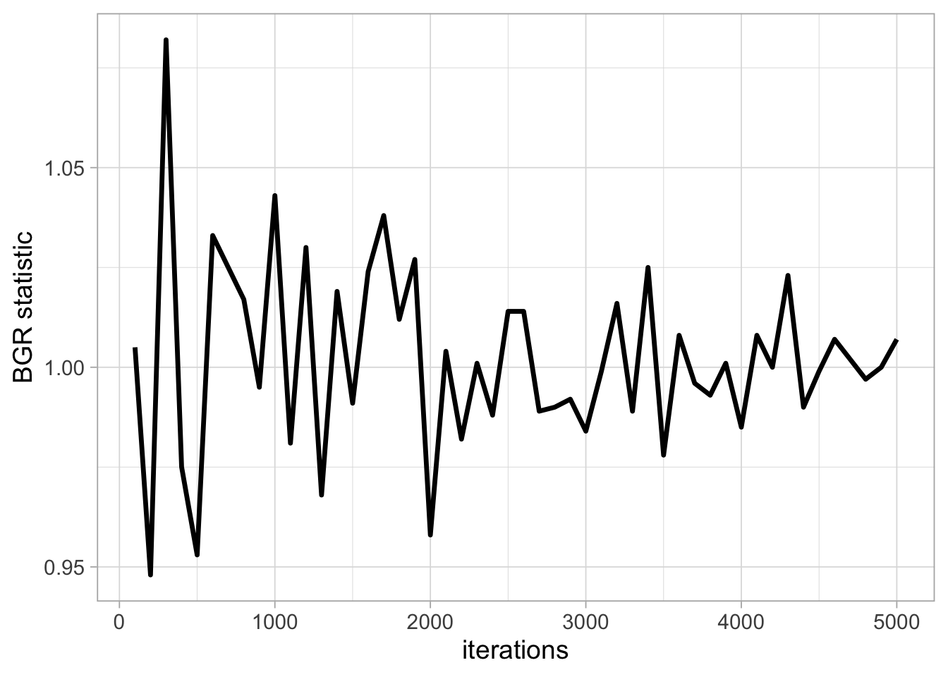
We get a value of the BGR statistic near 1 by up to 2000 iterations, which suggests that with 2000 iterations as a burn-in, there is no evidence of a lack of convergence.
It is important to bear in mind that a value near 1 for the BGR statistic is only a necessary but not sufficient condition for convergence. In other words, this diagnostic cannot tell you for sure that the Markov chain has achieved convergence, only that it has not.
1.6.2 Chain length
How long of a chain is needed to produce reliable parameter estimates? To answer this question, you need to keep in mind that successive steps in a Markov chain are not independent – this is usually referred to as autocorrelation. Ideally, we would like to keep autocorrelation as low as possible. Here again, trace plots are useful to diagnose issues with autocorrelation. Let’s get back to our survival example. The figure below shows trace plots for different values of the standard deviation (parameter away) of the normal proposal distribution we use to propose a candidate value (Section 1.5.3):
# inspired from
# https://bookdown.org/content/3686/markov-chain-monte-carlo.html

n_steps <- 10000

d <-
  tibble(away = c(0.1, 1, 10)) %>%
  mutate(accepted_traj = map(away,
                             metropolis,
                             steps = n_steps,
                             inits = 0.1)) %>%
  unnest(accepted_traj)

d <-
  d %>%
  mutate(proposal_sd = str_c("Proposal SD = ", away),
         iter        = rep(1:n_steps, times = 3))

trace <- d %>%
  ggplot(aes(y = accepted_traj, x = iter)) +
  geom_path(size = 1/4, color = "steelblue") +
  geom_point(size = 1/2, alpha = 1/2, color = "steelblue") +
  scale_y_continuous("survival",
                     breaks = 0:5 * 0.1,
                     limits = c(0.15, 0.5)) +
  scale_x_continuous("iterations",
                     breaks = seq(n_steps-n_steps*10/100,
                                  n_steps,
                                  by = 600),
                     limits = c(n_steps-n_steps*10/100,n_steps)) +
  facet_wrap(~proposal_sd, ncol = 3) +
  theme_light(base_size = 14)

trace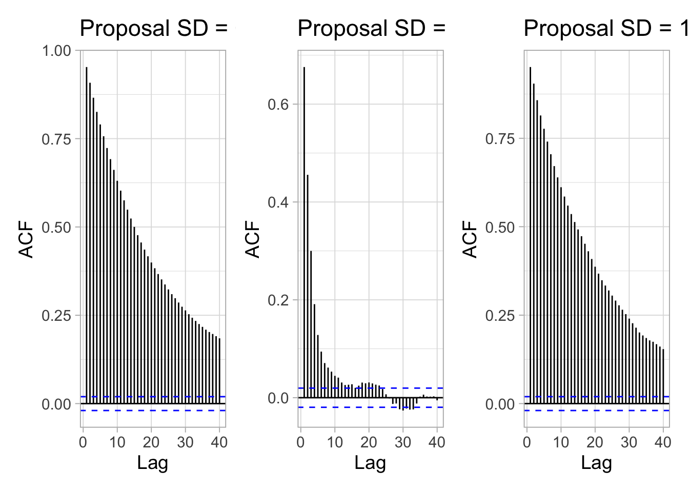
Small and big moves in the left and right panels provide high correlations between successive observations of the Markov chain, whereas a standard deviation of 1 in the center panel allows efficient exploration of the parameter space. The movement around the parameter space is referred to as mixing. Mixing is bad when the chain makes small and big moves, and good otherwise.
In addition to trace plots, autocorrelation function (ACF) plots are a convenient way of displaying the strength of autocorrelation in a given sample values. ACF plots provide the autocorrelation between successively sampled values separated by an increasing number of iterations, or lag. We obtain the autocorrelation function plots for different values of the standard deviation of the proposal distribution with the R forecast::ggAcf() function:
library(forecast)
mask <- d$proposal_sd=="Proposal SD = 0.1"
plot1 <- ggAcf(x = d$accepted_traj[mask]) + ggtitle("SD = 0.1")
mask <- d$proposal_sd=="Proposal SD = 1"
plot2 <- ggAcf(x = d$accepted_traj[mask]) + ggtitle("SD = 1")
mask <- d$proposal_sd=="Proposal SD = 10"
plot3 <- ggAcf(x = d$accepted_traj[mask]) + ggtitle("SD = 10")

library(patchwork)
(plot1 + plot2 + plot3)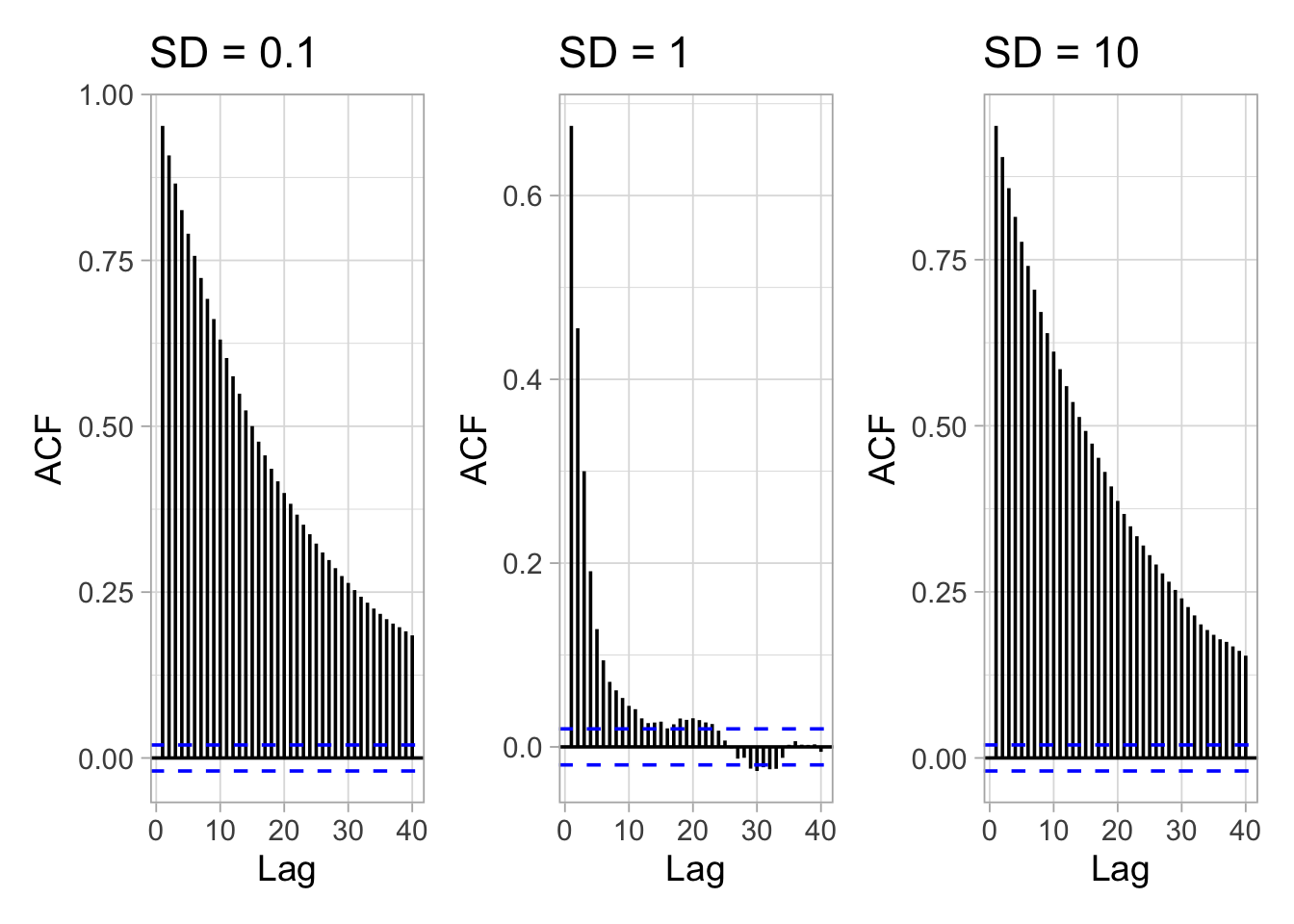
In the left and right panels, autocorrelation is strong, decreases slowly with increasing lag and mixing is bad. In the center panel, autocorrelation is weak, decreases rapidly with increasing lag and mixing is good.
Autocorrelation is not necessarily a big issue. Strongly correlated observations just require large sample sizes and therefore longer simulations. But how many iterations exactly? The effective sample size (n.eff) measures chain length while taking into account chain autocorrelation. You should check the n.eff of every parameter of interest, and of any interesting parameter combinations. In general, we need \(\text{n.eff} \geq 400\) independent steps to get reasonable Monte Carlo estimates of model parameters. In the animal survival example, n.eff can be calculated with the R coda::effectiveSize() function:
mask <- d$proposal_sd=="Proposal SD = 0.1"
neff1 <- coda::effectiveSize(d$accepted_traj[mask])
mask <- d$proposal_sd=="Proposal SD = 1"
neff2 <- coda::effectiveSize(d$accepted_traj[mask])
mask <- d$proposal_sd=="Proposal SD = 10"
neff3 <- coda::effectiveSize(d$accepted_traj[mask])
df <- tibble("Proposal SD" = c(0.1, 1, 10),
             "n.eff" = round(c(neff1, neff2, neff3)))
df
## # A tibble: 3 × 2
##   `Proposal SD` n.eff
##           <dbl> <dbl>
## 1           0.1   224
## 2           1    1934
## 3          10     230
As expected, n.eff is less than the number of MCMC iterations because of autocorrelation. Only when the standard deviation of the proposal distribution is 1 is the mixing good and we get a satisfying effective sample size.
1.6.3 What if you have issues of convergence?
When diagnosing MCMC convergence, you will (very) often run into troubles. In this section you will find some helpful tips I hope.
When mixing is bad and effective sample size is small, you may just need to increase burn-in and/or sample more. Using more informative priors might also make Markov chains converge faster by helping your MCMC sampler (e.g. the Metropolis algorithm) navigating more efficiently the parameter space. In the same spirit, picking better initial values for starting the chain does not harm. For doing that, a strategy consists in using estimates from a simpler model for which your MCMC chains do converge.
If convergence issues persist, often there is a problem with your model (also known as the folk theorem of statistical computing as stated by Andrew Gelman, see https://statmodeling.stat.columbia.edu/2008/05/13/the_folk_theore/). A bug in the code? A typo somewhere? A mistake in your maths? As often when coding is involved, the issue can be identified by removing complexities, and start with a simpler model until you find what the problem is.
A general advice is to see your model as a data generating tool in the first place, simulate data from it using some realistic values for the parameters, and try to recover these parameter values by fitting the model to the simulated data. Simulating from a model will help you understanding how it works, what it does not do, and the data you need to get reasonable parameter estimates (e.g. Chapter 3 and Section 7.4).
1.7 Summary
With the Bayes’ theorem, you update your beliefs (prior) with new data (likelihood) to get posterior beliefs (posterior): posterior \(\propto\) likelihood \(\times\) prior.
The idea of Markov chain Monte Carlo (MCMC) is to simulate values from a Markov chain which has a stationary distribution equal to the posterior distribution you’re after.
In practice, you run a Markov chain multiple times starting from over-dispersed initial values.
You discard iterations in an initial burn-in phase and achieve convergence when all chains reach the same regime.
From there, you run the chains long enough and proceed with calculating Monte Carlo estimates of numerical summaries (e.g. posterior means and credible intervals) for parameters.
1.8 Suggested reading
McCarthy (2007) and Kéry and Schaub (2011) are excellent introductions to Bayesian statistics for ecologists. The forthcoming second edition of the latter will also include NIMBLE code. See also Kéry and Kellner (2024).
For deeper insights, I recommend Gelman and Hill (2006) which analyse data using the frequentist and Bayesian approaches side-by-side. The book by McElreath (2020) is also an excellent read. The presentation of the Metropolis algorithm in Section 1.5.3 was inspired by Albert and Hu (2019). If you’d like to know more about Monte Carlo methods, the book Robert and Casella (2004) is a must (see also its R counterpart Robert and Casella 2010). See also Vehtari et al. (2021) for a discussion on \(\hat{R}\) and the effective sample size.
I also recommend Gelman et al. (2020) in which the authors offer a workflow for Bayesian analyses. They discuss model building, model comparison, model checking, model validation, model understanding and troubleshooting of computational problems.