Bayesian analyses made easy: GLMMs in R package brms
Here I illustrate how to fit GLMMs with the R package brms, and compare to Jags and lme4.
Motivation
I regularly give
a course on Bayesian statistics with R for non-specialists. To illustrate the course, we analyse data with
generalized linear, often mixed, models or GLMMs.
So far, I’ve been using Jags to fit these models. This requires some programming skills, like e.g. coding a loop, to be able to write down the model likelihood. Although students learn a lot from going through that process, it can be daunting.
This year, I thought I’d show them the
R package brms developed by
Paul-Christian Bürkner. In brief, brms allows fitting GLMMs (but not only) in a lme4-like syntax within the Bayesian framework and MCMC methods with Stan.
I’m not a Stan user, but it doesn’t matter. The
vignettes were more than enough to get me started. I also recommend the
list of blog posts about brms.
First things first, we load the packages we will need:
library(brms)
library(posterior) # tools for working with posterior and prior distributions
library(R2jags) # run Jags from within R
library(lme4) # fit GLMM in frequentist framework
Beta-Binomial model
The first example is about a survival experiment. We captured, marked and released 57 individuals (total) out of which 19 made it through the year (alive).
dat <- data.frame(alive = 19, total = 57)
dat
An obvious estimate of the probability of a binomial is the proportion of cases, $19/57 = 0.3333333$ here, but let’s use R built-in functions for the sake of illustration.
Maximum-likelihood estimation
To get an estimate of survival, we fit a logistic regression using the glm() function. The data are grouped (or aggregated), so we need to specify the number of alive and dead individuals as a two-column matrix on the left hand side of the model formula:
mle <- glm(cbind(alive, total - alive) ~ 1,
           family = binomial("logit"), # family = binomial("identity") would be more straightforward
           data = dat)
On the logit scale, survival is estimated at:
coef(mle) # logit scale
## (Intercept)
##  -0.6931472
After back-transformation using the reciprocal logit, we obtain:
plogis(coef(mle))
## (Intercept)
##   0.3333333
So far, so good.
Bayesian analysis with Jags
In Jags, you can fit this model with:
# model
betabin <- function(){
  alive ~ dbin(survival, total) # binomial likelihood
  logit(survival) <- beta # logit link
  beta ~ dnorm(0, 1/1.5) # prior
}
# data
datax <- list(total = 57,
              alive = 19)
# initial values
inits <- function() list(beta = rnorm(1, 0, sd = 1.5))
# parameter to monitor
params <- c("survival")
# run jags
bayes.jags <- jags(data = datax,
                      inits = inits,
                      parameters.to.save = params,
                      model.file = betabin,
                      n.chains = 2,
                      n.iter = 5000,
                      n.burnin = 1000,
                      n.thin = 1)
## Compiling model graph
##    Resolving undeclared variables
##    Allocating nodes
## Graph information:
##    Observed stochastic nodes: 1
##    Unobserved stochastic nodes: 1
##    Total graph size: 8
##
## Initializing model
# display results
bayes.jags
## Inference for Bugs model at "/var/folders/r7/j0wqj1k95vz8w44sdxzm986c0000gn/T//RtmpP7MZ1A/modela81d72dd23e2.txt", fit using jags,
##  2 chains, each with 5000 iterations (first 1000 discarded)
##  n.sims = 8000 iterations saved
##          mu.vect sd.vect  2.5%   25%   50%   75% 97.5%  Rhat n.eff
## survival   0.342   0.061 0.228 0.300 0.341 0.382 0.466 1.001  2600
## deviance   5.354   1.390 4.388 4.486 4.819 5.662 9.333 1.001  8000
##
## For each parameter, n.eff is a crude measure of effective sample size,
## and Rhat is the potential scale reduction factor (at convergence, Rhat=1).
##
## DIC info (using the rule, pD = var(deviance)/2)
## pD = 1.0 and DIC = 6.3
## DIC is an estimate of expected predictive error (lower deviance is better).
Bayesian analysis with brms
In brms, you write:
bayes.brms <- brm(alive | trials(total) ~ 1,
                  family = binomial("logit"), # binomial("identity") would be more straightforward
                  data = dat,
                  chains = 2, # nb of chains
                  iter = 5000, # nb of iterations, including burnin
                  warmup = 1000, # burnin
                  thin = 1) # thinning
## Running /Library/Frameworks/R.framework/Resources/bin/R CMD SHLIB foo.c
## clang -mmacosx-version-min=10.13 -I"/Library/Frameworks/R.framework/Resources/include" -DNDEBUG   -I"/Library/Frameworks/R.framework/Versions/4.1/Resources/library/Rcpp/include/"  -I"/Library/Frameworks/R.framework/Versions/4.1/Resources/library/RcppEigen/include/"  -I"/Library/Frameworks/R.framework/Versions/4.1/Resources/library/RcppEigen/include/unsupported"  -I"/Library/Frameworks/R.framework/Versions/4.1/Resources/library/BH/include" -I"/Library/Frameworks/R.framework/Versions/4.1/Resources/library/StanHeaders/include/src/"  -I"/Library/Frameworks/R.framework/Versions/4.1/Resources/library/StanHeaders/include/"  -I"/Library/Frameworks/R.framework/Versions/4.1/Resources/library/RcppParallel/include/"  -I"/Library/Frameworks/R.framework/Versions/4.1/Resources/library/rstan/include" -DEIGEN_NO_DEBUG  -DBOOST_DISABLE_ASSERTS  -DBOOST_PENDING_INTEGER_LOG2_HPP  -DSTAN_THREADS  -DBOOST_NO_AUTO_PTR  -include '/Library/Frameworks/R.framework/Versions/4.1/Resources/library/StanHeaders/include/stan/math/prim/mat/fun/Eigen.hpp'  -D_REENTRANT -DRCPP_PARALLEL_USE_TBB=1   -I/usr/local/include   -fPIC  -Wall -g -O2  -c foo.c -o foo.o
## In file included from <built-in>:1:
## In file included from /Library/Frameworks/R.framework/Versions/4.1/Resources/library/StanHeaders/include/stan/math/prim/mat/fun/Eigen.hpp:13:
## In file included from /Library/Frameworks/R.framework/Versions/4.1/Resources/library/RcppEigen/include/Eigen/Dense:1:
## In file included from /Library/Frameworks/R.framework/Versions/4.1/Resources/library/RcppEigen/include/Eigen/Core:88:
## /Library/Frameworks/R.framework/Versions/4.1/Resources/library/RcppEigen/include/Eigen/src/Core/util/Macros.h:628:1: error: unknown type name 'namespace'
## namespace Eigen {
## ^
## /Library/Frameworks/R.framework/Versions/4.1/Resources/library/RcppEigen/include/Eigen/src/Core/util/Macros.h:628:16: error: expected ';' after top level declarator
## namespace Eigen {
##                ^
##                ;
## In file included from <built-in>:1:
## In file included from /Library/Frameworks/R.framework/Versions/4.1/Resources/library/StanHeaders/include/stan/math/prim/mat/fun/Eigen.hpp:13:
## In file included from /Library/Frameworks/R.framework/Versions/4.1/Resources/library/RcppEigen/include/Eigen/Dense:1:
## /Library/Frameworks/R.framework/Versions/4.1/Resources/library/RcppEigen/include/Eigen/Core:96:10: fatal error: 'complex' file not found
## #include <complex>
##          ^~~~~~~~~
## 3 errors generated.
## make: *** [foo.o] Error 1
##
## SAMPLING FOR MODEL '782790eabbd10296f779d85fa03cf1e5' NOW (CHAIN 1).
## Chain 1:
## Chain 1: Gradient evaluation took 2e-05 seconds
## Chain 1: 1000 transitions using 10 leapfrog steps per transition would take 0.2 seconds.
## Chain 1: Adjust your expectations accordingly!
## Chain 1:
## Chain 1:
## Chain 1: Iteration:    1 / 5000 [  0%]  (Warmup)
## Chain 1: Iteration:  500 / 5000 [ 10%]  (Warmup)
## Chain 1: Iteration: 1000 / 5000 [ 20%]  (Warmup)
## Chain 1: Iteration: 1001 / 5000 [ 20%]  (Sampling)
## Chain 1: Iteration: 1500 / 5000 [ 30%]  (Sampling)
## Chain 1: Iteration: 2000 / 5000 [ 40%]  (Sampling)
## Chain 1: Iteration: 2500 / 5000 [ 50%]  (Sampling)
## Chain 1: Iteration: 3000 / 5000 [ 60%]  (Sampling)
## Chain 1: Iteration: 3500 / 5000 [ 70%]  (Sampling)
## Chain 1: Iteration: 4000 / 5000 [ 80%]  (Sampling)
## Chain 1: Iteration: 4500 / 5000 [ 90%]  (Sampling)
## Chain 1: Iteration: 5000 / 5000 [100%]  (Sampling)
## Chain 1:
## Chain 1:  Elapsed Time: 0.010358 seconds (Warm-up)
## Chain 1:                0.046464 seconds (Sampling)
## Chain 1:                0.056822 seconds (Total)
## Chain 1:
##
## SAMPLING FOR MODEL '782790eabbd10296f779d85fa03cf1e5' NOW (CHAIN 2).
## Chain 2:
## Chain 2: Gradient evaluation took 1.3e-05 seconds
## Chain 2: 1000 transitions using 10 leapfrog steps per transition would take 0.13 seconds.
## Chain 2: Adjust your expectations accordingly!
## Chain 2:
## Chain 2:
## Chain 2: Iteration:    1 / 5000 [  0%]  (Warmup)
## Chain 2: Iteration:  500 / 5000 [ 10%]  (Warmup)
## Chain 2: Iteration: 1000 / 5000 [ 20%]  (Warmup)
## Chain 2: Iteration: 1001 / 5000 [ 20%]  (Sampling)
## Chain 2: Iteration: 1500 / 5000 [ 30%]  (Sampling)
## Chain 2: Iteration: 2000 / 5000 [ 40%]  (Sampling)
## Chain 2: Iteration: 2500 / 5000 [ 50%]  (Sampling)
## Chain 2: Iteration: 3000 / 5000 [ 60%]  (Sampling)
## Chain 2: Iteration: 3500 / 5000 [ 70%]  (Sampling)
## Chain 2: Iteration: 4000 / 5000 [ 80%]  (Sampling)
## Chain 2: Iteration: 4500 / 5000 [ 90%]  (Sampling)
## Chain 2: Iteration: 5000 / 5000 [100%]  (Sampling)
## Chain 2:
## Chain 2:  Elapsed Time: 0.009763 seconds (Warm-up)
## Chain 2:                0.035949 seconds (Sampling)
## Chain 2:                0.045712 seconds (Total)
## Chain 2:
You can display the results:
bayes.brms
##  Family: binomial
##   Links: mu = logit
## Formula: alive | trials(total) ~ 1
##    Data: dat (Number of observations: 1)
##   Draws: 2 chains, each with iter = 5000; warmup = 1000; thin = 1;
##          total post-warmup draws = 8000
##
## Population-Level Effects:
##           Estimate Est.Error l-95% CI u-95% CI Rhat Bulk_ESS Tail_ESS
## Intercept    -0.69      0.28    -1.27    -0.14 1.00     3213     3572
##
## Draws were sampled using sampling(NUTS). For each parameter, Bulk_ESS
## and Tail_ESS are effective sample size measures, and Rhat is the potential
## scale reduction factor on split chains (at convergence, Rhat = 1).
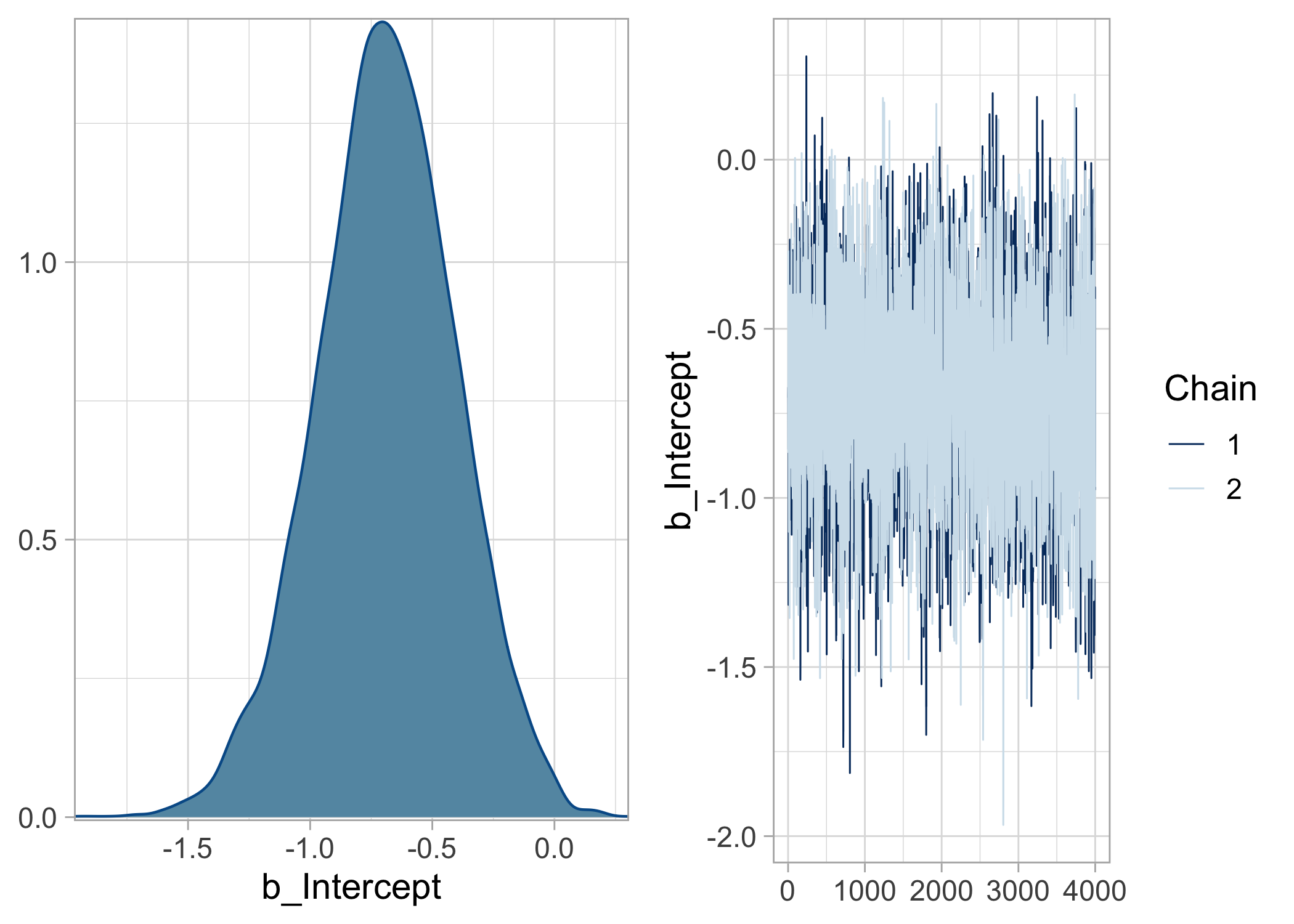
And visualize the posterior density and trace of survival (on the logit scale):
plot(bayes.brms)
To get survival on the $[0,1]$ scale, we extract the MCMC values, then apply the reciprocal logit function to each of these values, and summarize its posterior distribution:
draws_fit <- as_draws_matrix(bayes.brms)
draws_fit
## # A draws_matrix: 4000 iterations, 2 chains, and 2 variables
##     variable
## draw b_Intercept lp__
##   1        -0.70 -4.2
##   2        -0.67 -4.2
##   3        -0.86 -4.4
##   4        -0.80 -4.3
##   5        -1.32 -6.6
##   6        -0.57 -4.2
##   7        -0.51 -4.4
##   8        -0.56 -4.3
##   9        -0.69 -4.2
##   10       -0.41 -4.6
## # ... with 7990 more draws
summarize_draws(plogis(draws_fit[,1]))
What is the prior used by default?
prior_summary(bayes.brms)
What if I want to use the same prior as in Jags instead?
nlprior <- prior(normal(0, 1.5), class = "Intercept") # new prior
bayes.brms <- brm(alive | trials(total) ~ 1,
                  family = binomial("logit"),
                  data = dat,
                  prior = nlprior, # set prior by hand
                  chains = 2, # nb of chains
                  iter = 5000, # nb of iterations, including burnin
                  warmup = 1000, # burnin
                  thin = 1)
## Running /Library/Frameworks/R.framework/Resources/bin/R CMD SHLIB foo.c
## clang -mmacosx-version-min=10.13 -I"/Library/Frameworks/R.framework/Resources/include" -DNDEBUG   -I"/Library/Frameworks/R.framework/Versions/4.1/Resources/library/Rcpp/include/"  -I"/Library/Frameworks/R.framework/Versions/4.1/Resources/library/RcppEigen/include/"  -I"/Library/Frameworks/R.framework/Versions/4.1/Resources/library/RcppEigen/include/unsupported"  -I"/Library/Frameworks/R.framework/Versions/4.1/Resources/library/BH/include" -I"/Library/Frameworks/R.framework/Versions/4.1/Resources/library/StanHeaders/include/src/"  -I"/Library/Frameworks/R.framework/Versions/4.1/Resources/library/StanHeaders/include/"  -I"/Library/Frameworks/R.framework/Versions/4.1/Resources/library/RcppParallel/include/"  -I"/Library/Frameworks/R.framework/Versions/4.1/Resources/library/rstan/include" -DEIGEN_NO_DEBUG  -DBOOST_DISABLE_ASSERTS  -DBOOST_PENDING_INTEGER_LOG2_HPP  -DSTAN_THREADS  -DBOOST_NO_AUTO_PTR  -include '/Library/Frameworks/R.framework/Versions/4.1/Resources/library/StanHeaders/include/stan/math/prim/mat/fun/Eigen.hpp'  -D_REENTRANT -DRCPP_PARALLEL_USE_TBB=1   -I/usr/local/include   -fPIC  -Wall -g -O2  -c foo.c -o foo.o
## In file included from <built-in>:1:
## In file included from /Library/Frameworks/R.framework/Versions/4.1/Resources/library/StanHeaders/include/stan/math/prim/mat/fun/Eigen.hpp:13:
## In file included from /Library/Frameworks/R.framework/Versions/4.1/Resources/library/RcppEigen/include/Eigen/Dense:1:
## In file included from /Library/Frameworks/R.framework/Versions/4.1/Resources/library/RcppEigen/include/Eigen/Core:88:
## /Library/Frameworks/R.framework/Versions/4.1/Resources/library/RcppEigen/include/Eigen/src/Core/util/Macros.h:628:1: error: unknown type name 'namespace'
## namespace Eigen {
## ^
## /Library/Frameworks/R.framework/Versions/4.1/Resources/library/RcppEigen/include/Eigen/src/Core/util/Macros.h:628:16: error: expected ';' after top level declarator
## namespace Eigen {
##                ^
##                ;
## In file included from <built-in>:1:
## In file included from /Library/Frameworks/R.framework/Versions/4.1/Resources/library/StanHeaders/include/stan/math/prim/mat/fun/Eigen.hpp:13:
## In file included from /Library/Frameworks/R.framework/Versions/4.1/Resources/library/RcppEigen/include/Eigen/Dense:1:
## /Library/Frameworks/R.framework/Versions/4.1/Resources/library/RcppEigen/include/Eigen/Core:96:10: fatal error: 'complex' file not found
## #include <complex>
##          ^~~~~~~~~
## 3 errors generated.
## make: *** [foo.o] Error 1
##
## SAMPLING FOR MODEL '59dcc499a2b4c8a1b2c8f4e80e70fcce' NOW (CHAIN 1).
## Chain 1:
## Chain 1: Gradient evaluation took 1.8e-05 seconds
## Chain 1: 1000 transitions using 10 leapfrog steps per transition would take 0.18 seconds.
## Chain 1: Adjust your expectations accordingly!
## Chain 1:
## Chain 1:
## Chain 1: Iteration:    1 / 5000 [  0%]  (Warmup)
## Chain 1: Iteration:  500 / 5000 [ 10%]  (Warmup)
## Chain 1: Iteration: 1000 / 5000 [ 20%]  (Warmup)
## Chain 1: Iteration: 1001 / 5000 [ 20%]  (Sampling)
## Chain 1: Iteration: 1500 / 5000 [ 30%]  (Sampling)
## Chain 1: Iteration: 2000 / 5000 [ 40%]  (Sampling)
## Chain 1: Iteration: 2500 / 5000 [ 50%]  (Sampling)
## Chain 1: Iteration: 3000 / 5000 [ 60%]  (Sampling)
## Chain 1: Iteration: 3500 / 5000 [ 70%]  (Sampling)
## Chain 1: Iteration: 4000 / 5000 [ 80%]  (Sampling)
## Chain 1: Iteration: 4500 / 5000 [ 90%]  (Sampling)
## Chain 1: Iteration: 5000 / 5000 [100%]  (Sampling)
## Chain 1:
## Chain 1:  Elapsed Time: 0.00875 seconds (Warm-up)
## Chain 1:                0.03345 seconds (Sampling)
## Chain 1:                0.0422 seconds (Total)
## Chain 1:
##
## SAMPLING FOR MODEL '59dcc499a2b4c8a1b2c8f4e80e70fcce' NOW (CHAIN 2).
## Chain 2:
## Chain 2: Gradient evaluation took 5e-06 seconds
## Chain 2: 1000 transitions using 10 leapfrog steps per transition would take 0.05 seconds.
## Chain 2: Adjust your expectations accordingly!
## Chain 2:
## Chain 2:
## Chain 2: Iteration:    1 / 5000 [  0%]  (Warmup)
## Chain 2: Iteration:  500 / 5000 [ 10%]  (Warmup)
## Chain 2: Iteration: 1000 / 5000 [ 20%]  (Warmup)
## Chain 2: Iteration: 1001 / 5000 [ 20%]  (Sampling)
## Chain 2: Iteration: 1500 / 5000 [ 30%]  (Sampling)
## Chain 2: Iteration: 2000 / 5000 [ 40%]  (Sampling)
## Chain 2: Iteration: 2500 / 5000 [ 50%]  (Sampling)
## Chain 2: Iteration: 3000 / 5000 [ 60%]  (Sampling)
## Chain 2: Iteration: 3500 / 5000 [ 70%]  (Sampling)
## Chain 2: Iteration: 4000 / 5000 [ 80%]  (Sampling)
## Chain 2: Iteration: 4500 / 5000 [ 90%]  (Sampling)
## Chain 2: Iteration: 5000 / 5000 [100%]  (Sampling)
## Chain 2:
## Chain 2:  Elapsed Time: 0.009788 seconds (Warm-up)
## Chain 2:                0.036797 seconds (Sampling)
## Chain 2:                0.046585 seconds (Total)
## Chain 2:
Double-check the prior that was used:
prior_summary(bayes.brms)
Logistic regression with covariates
In this example, we ask whether annual variation in white stork breeding success can be explained by rainfall in the wintering area. Breeding success is measured by the ratio of the number of chicks over the number of pairs.
nbchicks <- c(151,105,73,107,113,87,77,108,118,122,112,120,122,89,69,71,53,41,53,31,35,14,18)
nbpairs <- c(173,164,103,113,122,112,98,121,132,136,133,137,145,117,90,80,67,54,58,39,42,23,23)
rain <- c(67,52,88,61,32,36,72,43,92,32,86,28,57,55,66,26,28,96,48,90,86,78,87)
dat <- data.frame(nbchicks = nbchicks,
                  nbpairs = nbpairs,
                  rain = (rain - mean(rain))/sd(rain)) # standardized rainfall
The data are grouped.
Maximum-likelihood estimation
You can get maximum likelihood estimates with:
mle <- glm(cbind(nbchicks, nbpairs - nbchicks) ~ rain,
           family = binomial("logit"),
           data = dat)
summary(mle)
##
## Call:
## glm(formula = cbind(nbchicks, nbpairs - nbchicks) ~ rain, family = binomial("logit"),
##     data = dat)
##
## Deviance Residuals:
##     Min       1Q   Median       3Q      Max
## -5.9630  -1.3354   0.3929   1.6168   3.8800
##
## Coefficients:
##             Estimate Std. Error z value Pr(>|z|)
## (Intercept)  1.55436    0.05565  27.931   <2e-16 ***
## rain        -0.14857    0.05993  -2.479   0.0132 *
## ---
## Signif. codes:  0 '***' 0.001 '**' 0.01 '*' 0.05 '.' 0.1 ' ' 1
##
## (Dispersion parameter for binomial family taken to be 1)
##
##     Null deviance: 109.25  on 22  degrees of freedom
## Residual deviance: 103.11  on 21  degrees of freedom
## AIC: 205.84
##
## Number of Fisher Scoring iterations: 4
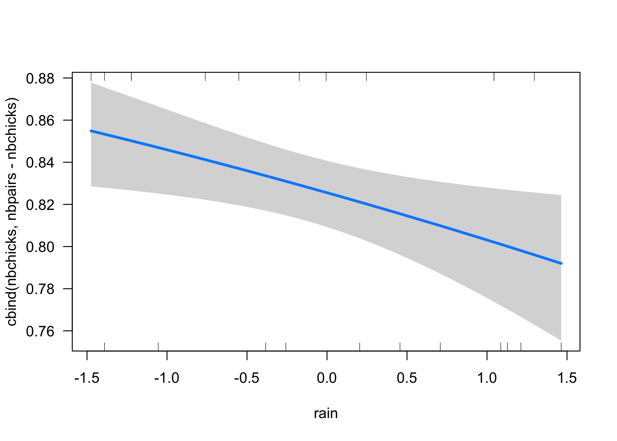
There is a negative effect of rainfall on breeding success:
visreg::visreg(mle, scale = "response")
Bayesian analysis with Jags
In Jags, we can fit the same model:
# data
dat <- list(N = 23, # nb of years
            nbchicks = nbchicks,
            nbpairs = nbpairs,
            rain = (rain - mean(rain))/sd(rain)) # standardized rainfall

# define model
logistic <- function() {
  # likelihood
  for(i in 1:N){ # loop over years
    nbchicks[i] ~ dbin(p[i], nbpairs[i]) # binomial likelihood
    logit(p[i]) <- a + b.rain * rain[i] # prob success is linear fn of rainfall on logit scale
  }
  # priors
  a ~ dnorm(0,0.01) # intercept
  b.rain ~ dnorm(0,0.01) # slope for rainfall
}

# function that generates initial values
inits <- function() list(a = rnorm(n = 1, mean = 0, sd = 5),
                         b.rain = rnorm(n = 1, mean = 0, sd = 5))

# specify parameters that need to be estimated
parameters <- c("a", "b.rain")

# run Jags
bayes.jags <- jags(data = dat,
               inits = inits,
               parameters.to.save = parameters,
               model.file = logistic,
               n.chains = 2,
               n.iter = 5000, # includes burn-in!
               n.burnin = 1000)
## Compiling model graph
##    Resolving undeclared variables
##    Allocating nodes
## Graph information:
##    Observed stochastic nodes: 23
##    Unobserved stochastic nodes: 2
##    Total graph size: 134
##
## Initializing model
# display results
bayes.jags
## Inference for Bugs model at "/var/folders/r7/j0wqj1k95vz8w44sdxzm986c0000gn/T//RtmpP7MZ1A/modela81d1b01bd3f.txt", fit using jags,
##  2 chains, each with 5000 iterations (first 1000 discarded), n.thin = 4
##  n.sims = 2000 iterations saved
##          mu.vect sd.vect    2.5%     25%     50%     75%   97.5%  Rhat n.eff
## a          1.546   0.163   1.439   1.514   1.552   1.588   1.657 1.182  2000
## b.rain    -0.152   0.121  -0.275  -0.190  -0.148  -0.106  -0.033 1.129  2000
## deviance 213.612 330.910 201.899 202.434 203.197 204.689 209.169 1.121  2000
##
## For each parameter, n.eff is a crude measure of effective sample size,
## and Rhat is the potential scale reduction factor (at convergence, Rhat=1).
##
## DIC info (using the rule, pD = var(deviance)/2)
## pD = 54753.9 and DIC = 54967.5
## DIC is an estimate of expected predictive error (lower deviance is better).
Bayesian analysis with brms
With brms, we write:
bayes.brms <- brm(nbchicks | trials(nbpairs) ~ rain,
                  family = binomial("logit"),
                  data = dat,
                  chains = 2, # nb of chains
                  iter = 5000, # nb of iterations, including burnin
                  warmup = 1000, # burnin
                  thin = 1)
## Running /Library/Frameworks/R.framework/Resources/bin/R CMD SHLIB foo.c
## clang -mmacosx-version-min=10.13 -I"/Library/Frameworks/R.framework/Resources/include" -DNDEBUG   -I"/Library/Frameworks/R.framework/Versions/4.1/Resources/library/Rcpp/include/"  -I"/Library/Frameworks/R.framework/Versions/4.1/Resources/library/RcppEigen/include/"  -I"/Library/Frameworks/R.framework/Versions/4.1/Resources/library/RcppEigen/include/unsupported"  -I"/Library/Frameworks/R.framework/Versions/4.1/Resources/library/BH/include" -I"/Library/Frameworks/R.framework/Versions/4.1/Resources/library/StanHeaders/include/src/"  -I"/Library/Frameworks/R.framework/Versions/4.1/Resources/library/StanHeaders/include/"  -I"/Library/Frameworks/R.framework/Versions/4.1/Resources/library/RcppParallel/include/"  -I"/Library/Frameworks/R.framework/Versions/4.1/Resources/library/rstan/include" -DEIGEN_NO_DEBUG  -DBOOST_DISABLE_ASSERTS  -DBOOST_PENDING_INTEGER_LOG2_HPP  -DSTAN_THREADS  -DBOOST_NO_AUTO_PTR  -include '/Library/Frameworks/R.framework/Versions/4.1/Resources/library/StanHeaders/include/stan/math/prim/mat/fun/Eigen.hpp'  -D_REENTRANT -DRCPP_PARALLEL_USE_TBB=1   -I/usr/local/include   -fPIC  -Wall -g -O2  -c foo.c -o foo.o
## In file included from <built-in>:1:
## In file included from /Library/Frameworks/R.framework/Versions/4.1/Resources/library/StanHeaders/include/stan/math/prim/mat/fun/Eigen.hpp:13:
## In file included from /Library/Frameworks/R.framework/Versions/4.1/Resources/library/RcppEigen/include/Eigen/Dense:1:
## In file included from /Library/Frameworks/R.framework/Versions/4.1/Resources/library/RcppEigen/include/Eigen/Core:88:
## /Library/Frameworks/R.framework/Versions/4.1/Resources/library/RcppEigen/include/Eigen/src/Core/util/Macros.h:628:1: error: unknown type name 'namespace'
## namespace Eigen {
## ^
## /Library/Frameworks/R.framework/Versions/4.1/Resources/library/RcppEigen/include/Eigen/src/Core/util/Macros.h:628:16: error: expected ';' after top level declarator
## namespace Eigen {
##                ^
##                ;
## In file included from <built-in>:1:
## In file included from /Library/Frameworks/R.framework/Versions/4.1/Resources/library/StanHeaders/include/stan/math/prim/mat/fun/Eigen.hpp:13:
## In file included from /Library/Frameworks/R.framework/Versions/4.1/Resources/library/RcppEigen/include/Eigen/Dense:1:
## /Library/Frameworks/R.framework/Versions/4.1/Resources/library/RcppEigen/include/Eigen/Core:96:10: fatal error: 'complex' file not found
## #include <complex>
##          ^~~~~~~~~
## 3 errors generated.
## make: *** [foo.o] Error 1
##
## SAMPLING FOR MODEL '70a68f0c53365768853c2791038e6352' NOW (CHAIN 1).
## Chain 1:
## Chain 1: Gradient evaluation took 4.7e-05 seconds
## Chain 1: 1000 transitions using 10 leapfrog steps per transition would take 0.47 seconds.
## Chain 1: Adjust your expectations accordingly!
## Chain 1:
## Chain 1:
## Chain 1: Iteration:    1 / 5000 [  0%]  (Warmup)
## Chain 1: Iteration:  500 / 5000 [ 10%]  (Warmup)
## Chain 1: Iteration: 1000 / 5000 [ 20%]  (Warmup)
## Chain 1: Iteration: 1001 / 5000 [ 20%]  (Sampling)
## Chain 1: Iteration: 1500 / 5000 [ 30%]  (Sampling)
## Chain 1: Iteration: 2000 / 5000 [ 40%]  (Sampling)
## Chain 1: Iteration: 2500 / 5000 [ 50%]  (Sampling)
## Chain 1: Iteration: 3000 / 5000 [ 60%]  (Sampling)
## Chain 1: Iteration: 3500 / 5000 [ 70%]  (Sampling)
## Chain 1: Iteration: 4000 / 5000 [ 80%]  (Sampling)
## Chain 1: Iteration: 4500 / 5000 [ 90%]  (Sampling)
## Chain 1: Iteration: 5000 / 5000 [100%]  (Sampling)
## Chain 1:
## Chain 1:  Elapsed Time: 0.035213 seconds (Warm-up)
## Chain 1:                0.131663 seconds (Sampling)
## Chain 1:                0.166876 seconds (Total)
## Chain 1:
##
## SAMPLING FOR MODEL '70a68f0c53365768853c2791038e6352' NOW (CHAIN 2).
## Chain 2:
## Chain 2: Gradient evaluation took 1.4e-05 seconds
## Chain 2: 1000 transitions using 10 leapfrog steps per transition would take 0.14 seconds.
## Chain 2: Adjust your expectations accordingly!
## Chain 2:
## Chain 2:
## Chain 2: Iteration:    1 / 5000 [  0%]  (Warmup)
## Chain 2: Iteration:  500 / 5000 [ 10%]  (Warmup)
## Chain 2: Iteration: 1000 / 5000 [ 20%]  (Warmup)
## Chain 2: Iteration: 1001 / 5000 [ 20%]  (Sampling)
## Chain 2: Iteration: 1500 / 5000 [ 30%]  (Sampling)
## Chain 2: Iteration: 2000 / 5000 [ 40%]  (Sampling)
## Chain 2: Iteration: 2500 / 5000 [ 50%]  (Sampling)
## Chain 2: Iteration: 3000 / 5000 [ 60%]  (Sampling)
## Chain 2: Iteration: 3500 / 5000 [ 70%]  (Sampling)
## Chain 2: Iteration: 4000 / 5000 [ 80%]  (Sampling)
## Chain 2: Iteration: 4500 / 5000 [ 90%]  (Sampling)
## Chain 2: Iteration: 5000 / 5000 [100%]  (Sampling)
## Chain 2:
## Chain 2:  Elapsed Time: 0.033715 seconds (Warm-up)
## Chain 2:                0.15264 seconds (Sampling)
## Chain 2:                0.186355 seconds (Total)
## Chain 2:
Display results:
bayes.brms
##  Family: binomial
##   Links: mu = logit
## Formula: nbchicks | trials(nbpairs) ~ rain
##    Data: dat (Number of observations: 23)
##   Draws: 2 chains, each with iter = 5000; warmup = 1000; thin = 1;
##          total post-warmup draws = 8000
##
## Population-Level Effects:
##           Estimate Est.Error l-95% CI u-95% CI Rhat Bulk_ESS Tail_ESS
## Intercept     1.56      0.06     1.45     1.67 1.00     6907     5043
## rain         -0.15      0.06    -0.27    -0.03 1.00     7193     5067
##
## Draws were sampled using sampling(NUTS). For each parameter, Bulk_ESS
## and Tail_ESS are effective sample size measures, and Rhat is the potential
## scale reduction factor on split chains (at convergence, Rhat = 1).
Visualize:
plot(bayes.brms)
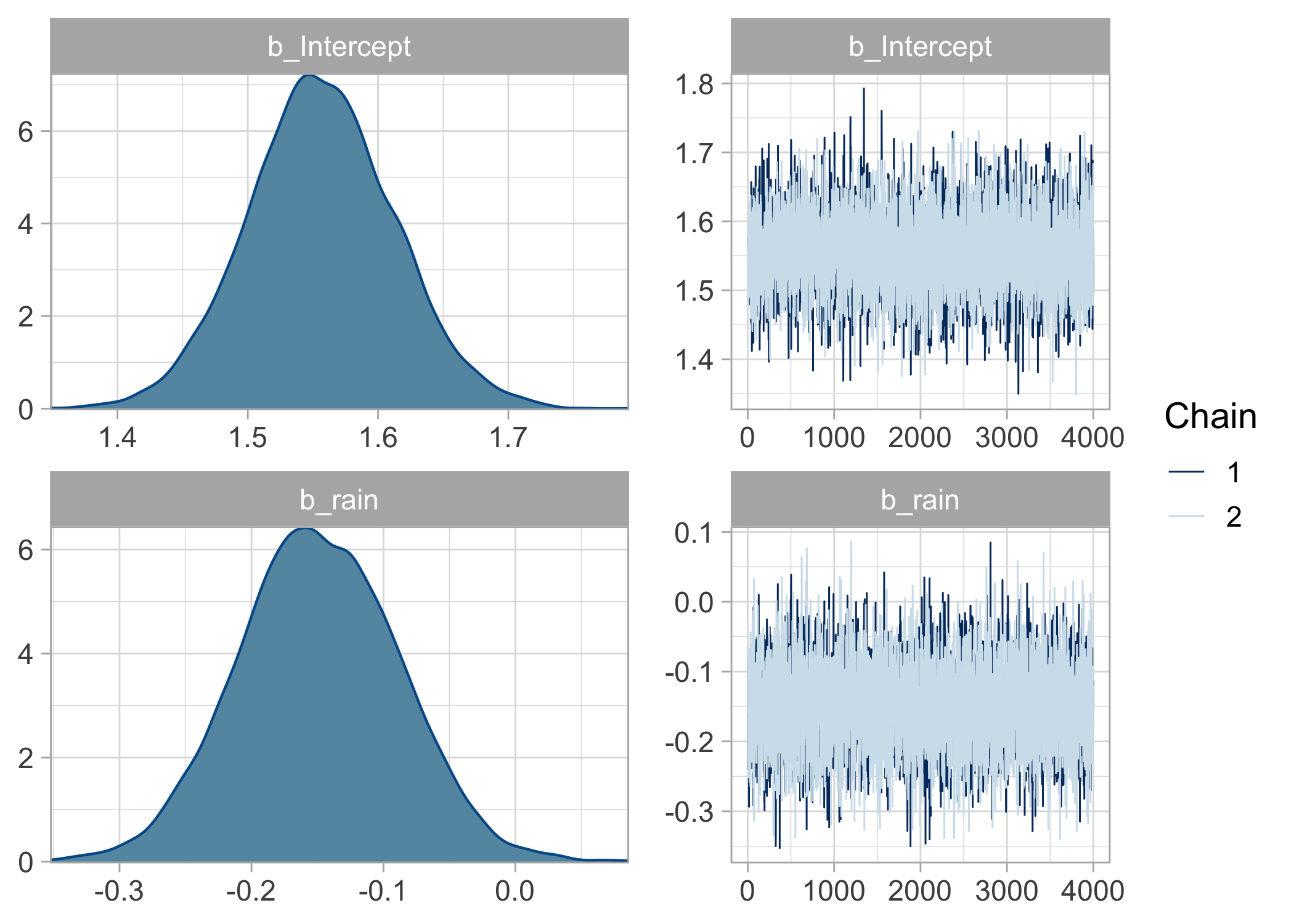
We can also calculate the posterior probability of the rainfall effect being below zero with the hypothesis() function:
hypothesis(bayes.brms, 'rain < 0')
## Hypothesis Tests for class b:
##   Hypothesis Estimate Est.Error CI.Lower CI.Upper Evid.Ratio Post.Prob Star
## 1 (rain) < 0    -0.15      0.06    -0.25    -0.05     116.65      0.99    *
## ---
## 'CI': 90%-CI for one-sided and 95%-CI for two-sided hypotheses.
## '*': For one-sided hypotheses, the posterior probability exceeds 95%;
## for two-sided hypotheses, the value tested against lies outside the 95%-CI.
## Posterior probabilities of point hypotheses assume equal prior probabilities.
These results confirm the important negative effect of rainfall on breeding success.
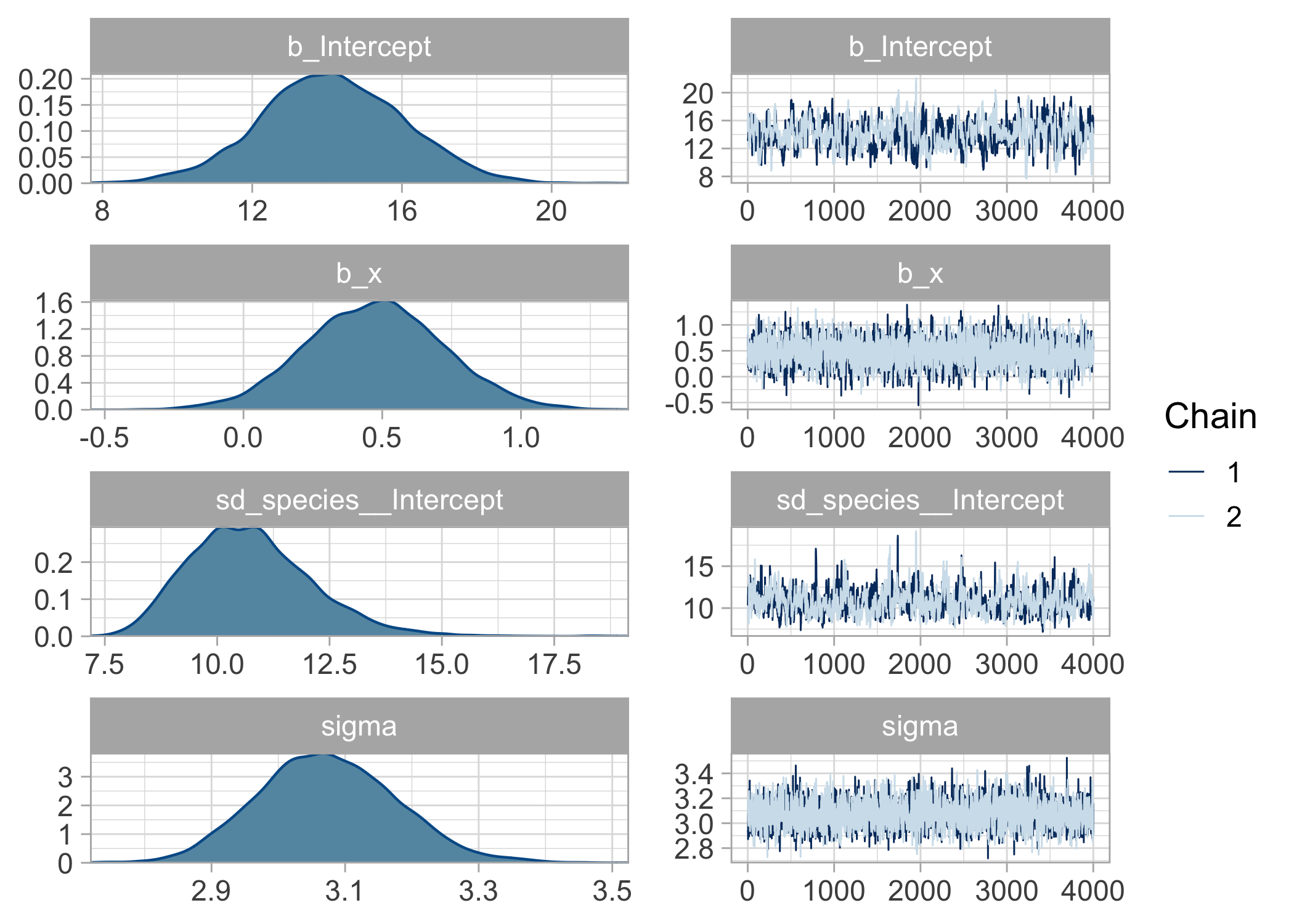
Linear mixed model
In this example, we have several measurements for 33 Mediterranean plant species, specifically number of seeds and biomass. We ask whether there is a linear relationship between these two variables that would hold for all species.
Read in data, directly from the course website:
df <- read_csv2("https://raw.githubusercontent.com/oliviergimenez/bayesian-stats-with-R/master/slides/dat/VMG.csv")
df
Use relevant format for columns species Sp and biomass Vm:
df$Sp <- as_factor(df$Sp)
df$Vm <- as.numeric(df$Vm)
Define numeric vector of species, for nested indexing in Jags:
species <- as.numeric(df$Sp)
Define response variable, number of seeds:
y <- log(df$NGrTotest)
Standardize explanatory variable, biomass
x <- (df$Vm - mean(df$Vm))/sd(df$Vm)
Now build dataset:
dat <- data.frame(y = y, x = x, species = species)
Maximum-likelihood estimation
You can get maximum likelihood estimates for a linear regression of number of seeds on biomass with a species random effect on the intercept (partial pooling):
mle <- lmer(y ~ x + (1 | species), data = dat)
summary(mle)
## Linear mixed model fit by REML ['lmerMod']
## Formula: y ~ x + (1 | species)
##    Data: dat
##
## REML criterion at convergence: 2642.5
##
## Scaled residuals:
##     Min      1Q  Median      3Q     Max
## -4.6761 -0.2704 -0.0120  0.2900  7.3163
##
## Random effects:
##  Groups   Name        Variance Std.Dev.
##  species  (Intercept) 113.146  10.637
##  Residual               9.373   3.062
## Number of obs: 488, groups:  species, 33
##
## Fixed effects:
##             Estimate Std. Error t value
## (Intercept)  14.5258     1.8574   7.821
## x             0.4779     0.2421   1.974
##
## Correlation of Fixed Effects:
##   (Intr)
## x 0.002
Bayesian analysis with Jags
In Jags, you would use:
# partial pooling model
partial_pooling <- function(){
  # likelihood
  for(i in 1:n){
    y[i] ~ dnorm(mu[i], tau.y)
    mu[i] <- a[species[i]] + b * x[i]
  }
  for (j in 1:nbspecies){
    a[j] ~ dnorm(mu.a, tau.a)
  }
  # priors
  tau.y <- 1 / (sigma.y * sigma.y)
  sigma.y ~ dunif(0,100)
  mu.a ~ dnorm(0,0.01)
  tau.a <- 1 / (sigma.a * sigma.a)
  sigma.a ~ dunif(0,100)
  b ~ dnorm(0,0.01)
}

# data
mydata <- list(y = y,
               x = x,
               n = length(y),
               species = species,
               nbspecies = length(levels(df$Sp)))

# initial values
inits <- function() list(mu.a = rnorm(1,0,5),
                         sigma.a = runif(0,0,10),
                         b = rnorm(1,0,5),
                         sigma.y = runif(0,0,10))

# parameters to monitor
params <- c("mu.a", "sigma.a", "b", "sigma.y")

# call jags to fit model
bayes.jags <- jags(data = mydata,
                   inits = inits,
                   parameters.to.save = params,
                   model.file = partial_pooling,
                   n.chains = 2,
                   n.iter = 5000,
                   n.burnin = 1000,
                   n.thin = 1)
## Compiling model graph
##    Resolving undeclared variables
##    Allocating nodes
## Graph information:
##    Observed stochastic nodes: 488
##    Unobserved stochastic nodes: 37
##    Total graph size: 2484
##
## Initializing model
bayes.jags
## Inference for Bugs model at "/var/folders/r7/j0wqj1k95vz8w44sdxzm986c0000gn/T//RtmpP7MZ1A/modela81d7639dc1c.txt", fit using jags,
##  2 chains, each with 5000 iterations (first 1000 discarded)
##  n.sims = 8000 iterations saved
##           mu.vect sd.vect     2.5%      25%      50%      75%    97.5%  Rhat
## b           0.476   0.244   -0.005    0.314    0.472    0.638    0.964 1.001
## mu.a       14.025   1.916   10.146   12.774   14.009   15.299   17.760 1.001
## sigma.a    11.094   1.465    8.696   10.039   10.934   11.952   14.330 1.001
## sigma.y     3.072   0.101    2.884    3.002    3.069    3.138    3.277 1.001
## deviance 2478.206   8.704 2463.096 2472.022 2477.521 2483.650 2497.107 1.001
##          n.eff
## b         8000
## mu.a      8000
## sigma.a   8000
## sigma.y   8000
## deviance  8000
##
## For each parameter, n.eff is a crude measure of effective sample size,
## and Rhat is the potential scale reduction factor (at convergence, Rhat=1).
##
## DIC info (using the rule, pD = var(deviance)/2)
## pD = 37.9 and DIC = 2516.1
## DIC is an estimate of expected predictive error (lower deviance is better).
Bayesian analysis with brms
In brms, you write:
bayes.brms <- brm(y ~ x + (1 | species),
                  data = dat,
                  chains = 2, # nb of chains
                  iter = 5000, # nb of iterations, including burnin
                  warmup = 1000, # burnin
                  thin = 1)
## Running /Library/Frameworks/R.framework/Resources/bin/R CMD SHLIB foo.c
## clang -mmacosx-version-min=10.13 -I"/Library/Frameworks/R.framework/Resources/include" -DNDEBUG   -I"/Library/Frameworks/R.framework/Versions/4.1/Resources/library/Rcpp/include/"  -I"/Library/Frameworks/R.framework/Versions/4.1/Resources/library/RcppEigen/include/"  -I"/Library/Frameworks/R.framework/Versions/4.1/Resources/library/RcppEigen/include/unsupported"  -I"/Library/Frameworks/R.framework/Versions/4.1/Resources/library/BH/include" -I"/Library/Frameworks/R.framework/Versions/4.1/Resources/library/StanHeaders/include/src/"  -I"/Library/Frameworks/R.framework/Versions/4.1/Resources/library/StanHeaders/include/"  -I"/Library/Frameworks/R.framework/Versions/4.1/Resources/library/RcppParallel/include/"  -I"/Library/Frameworks/R.framework/Versions/4.1/Resources/library/rstan/include" -DEIGEN_NO_DEBUG  -DBOOST_DISABLE_ASSERTS  -DBOOST_PENDING_INTEGER_LOG2_HPP  -DSTAN_THREADS  -DBOOST_NO_AUTO_PTR  -include '/Library/Frameworks/R.framework/Versions/4.1/Resources/library/StanHeaders/include/stan/math/prim/mat/fun/Eigen.hpp'  -D_REENTRANT -DRCPP_PARALLEL_USE_TBB=1   -I/usr/local/include   -fPIC  -Wall -g -O2  -c foo.c -o foo.o
## In file included from <built-in>:1:
## In file included from /Library/Frameworks/R.framework/Versions/4.1/Resources/library/StanHeaders/include/stan/math/prim/mat/fun/Eigen.hpp:13:
## In file included from /Library/Frameworks/R.framework/Versions/4.1/Resources/library/RcppEigen/include/Eigen/Dense:1:
## In file included from /Library/Frameworks/R.framework/Versions/4.1/Resources/library/RcppEigen/include/Eigen/Core:88:
## /Library/Frameworks/R.framework/Versions/4.1/Resources/library/RcppEigen/include/Eigen/src/Core/util/Macros.h:628:1: error: unknown type name 'namespace'
## namespace Eigen {
## ^
## /Library/Frameworks/R.framework/Versions/4.1/Resources/library/RcppEigen/include/Eigen/src/Core/util/Macros.h:628:16: error: expected ';' after top level declarator
## namespace Eigen {
##                ^
##                ;
## In file included from <built-in>:1:
## In file included from /Library/Frameworks/R.framework/Versions/4.1/Resources/library/StanHeaders/include/stan/math/prim/mat/fun/Eigen.hpp:13:
## In file included from /Library/Frameworks/R.framework/Versions/4.1/Resources/library/RcppEigen/include/Eigen/Dense:1:
## /Library/Frameworks/R.framework/Versions/4.1/Resources/library/RcppEigen/include/Eigen/Core:96:10: fatal error: 'complex' file not found
## #include <complex>
##          ^~~~~~~~~
## 3 errors generated.
## make: *** [foo.o] Error 1
##
## SAMPLING FOR MODEL 'c7dcb37f6d55803a5216866e78a4a476' NOW (CHAIN 1).
## Chain 1:
## Chain 1: Gradient evaluation took 0.000102 seconds
## Chain 1: 1000 transitions using 10 leapfrog steps per transition would take 1.02 seconds.
## Chain 1: Adjust your expectations accordingly!
## Chain 1:
## Chain 1:
## Chain 1: Iteration:    1 / 5000 [  0%]  (Warmup)
## Chain 1: Iteration:  500 / 5000 [ 10%]  (Warmup)
## Chain 1: Iteration: 1000 / 5000 [ 20%]  (Warmup)
## Chain 1: Iteration: 1001 / 5000 [ 20%]  (Sampling)
## Chain 1: Iteration: 1500 / 5000 [ 30%]  (Sampling)
## Chain 1: Iteration: 2000 / 5000 [ 40%]  (Sampling)
## Chain 1: Iteration: 2500 / 5000 [ 50%]  (Sampling)
## Chain 1: Iteration: 3000 / 5000 [ 60%]  (Sampling)
## Chain 1: Iteration: 3500 / 5000 [ 70%]  (Sampling)
## Chain 1: Iteration: 4000 / 5000 [ 80%]  (Sampling)
## Chain 1: Iteration: 4500 / 5000 [ 90%]  (Sampling)
## Chain 1: Iteration: 5000 / 5000 [100%]  (Sampling)
## Chain 1:
## Chain 1:  Elapsed Time: 0.656886 seconds (Warm-up)
## Chain 1:                3.37389 seconds (Sampling)
## Chain 1:                4.03077 seconds (Total)
## Chain 1:
##
## SAMPLING FOR MODEL 'c7dcb37f6d55803a5216866e78a4a476' NOW (CHAIN 2).
## Chain 2:
## Chain 2: Gradient evaluation took 2.7e-05 seconds
## Chain 2: 1000 transitions using 10 leapfrog steps per transition would take 0.27 seconds.
## Chain 2: Adjust your expectations accordingly!
## Chain 2:
## Chain 2:
## Chain 2: Iteration:    1 / 5000 [  0%]  (Warmup)
## Chain 2: Iteration:  500 / 5000 [ 10%]  (Warmup)
## Chain 2: Iteration: 1000 / 5000 [ 20%]  (Warmup)
## Chain 2: Iteration: 1001 / 5000 [ 20%]  (Sampling)
## Chain 2: Iteration: 1500 / 5000 [ 30%]  (Sampling)
## Chain 2: Iteration: 2000 / 5000 [ 40%]  (Sampling)
## Chain 2: Iteration: 2500 / 5000 [ 50%]  (Sampling)
## Chain 2: Iteration: 3000 / 5000 [ 60%]  (Sampling)
## Chain 2: Iteration: 3500 / 5000 [ 70%]  (Sampling)
## Chain 2: Iteration: 4000 / 5000 [ 80%]  (Sampling)
## Chain 2: Iteration: 4500 / 5000 [ 90%]  (Sampling)
## Chain 2: Iteration: 5000 / 5000 [100%]  (Sampling)
## Chain 2:
## Chain 2:  Elapsed Time: 0.593596 seconds (Warm-up)
## Chain 2:                2.34578 seconds (Sampling)
## Chain 2:                2.93937 seconds (Total)
## Chain 2:
Display the results:
bayes.brms
##  Family: gaussian
##   Links: mu = identity; sigma = identity
## Formula: y ~ x + (1 | species)
##    Data: dat (Number of observations: 488)
##   Draws: 2 chains, each with iter = 5000; warmup = 1000; thin = 1;
##          total post-warmup draws = 8000
##
## Group-Level Effects:
## ~species (Number of levels: 33)
##               Estimate Est.Error l-95% CI u-95% CI Rhat Bulk_ESS Tail_ESS
## sd(Intercept)    10.74      1.39     8.45    13.78 1.00      427      943
##
## Population-Level Effects:
##           Estimate Est.Error l-95% CI u-95% CI Rhat Bulk_ESS Tail_ESS
## Intercept    14.13      1.90    10.31    17.86 1.01      331      580
## x             0.47      0.25    -0.00     0.97 1.00     2317     3382
##
## Family Specific Parameters:
##       Estimate Est.Error l-95% CI u-95% CI Rhat Bulk_ESS Tail_ESS
## sigma     3.07      0.10     2.88     3.28 1.00     2667     3408
##
## Draws were sampled using sampling(NUTS). For each parameter, Bulk_ESS
## and Tail_ESS are effective sample size measures, and Rhat is the potential
## scale reduction factor on split chains (at convergence, Rhat = 1).
You can extract a block of fixed effects:
summary(bayes.brms)$fixed
And a block of random effects:
summary(bayes.brms)$random
## $species
##               Estimate Est.Error l-95% CI u-95% CI     Rhat Bulk_ESS Tail_ESS
## sd(Intercept) 10.74273  1.388061 8.454543   13.776 1.001916 426.9568 943.1178
And visualize:
plot(bayes.brms)
GLMM with Poisson distribution
This example is from Jason Matthiopoulos’ excellent book How to be a quantitative ecologist. A survey of a coral reef uses 10 predefined linear transects covered by divers once every week. The response variable of interest is the abundance of a particular species of anemone as a function of water temperature. Counts of anemones are recorded at 20 regular line segments along the transect.
Let’s simulate some data:
set.seed(666)
transects <- 10
data <- NULL
for (tr in 1:transects){
  # random effect (intercept)
  ref <- rnorm(1,0,.5)
  # water temperature gradient
  t <- runif(1, 18,22) + runif(1,-.2,0.2)*1:20
  # Anemone gradient (expected response)
  ans <- exp(ref -14 + 1.8 * t - 0.045 * t^2)
  # actual counts on 20 segments of the current transect
  an <- rpois(20, ans)
  data <- rbind(data, cbind(rep(tr, 20), t, an))
}

data <- data.frame(Transect = data[,1],
                   Temperature = data[,2],
                   Anemones = data[,3])
Standardize temperature:
boo <- data$Temperature
data$Temp <- (boo - mean(boo)) / sd(boo)
head(data)
Maximum-likelihood estimation
With lme4, you write:
fit_lme4 <- glmer(Anemones ~ Temp + I(Temp^2) + (1 | Transect),
                  data = data,
                  family = poisson)
summary(fit_lme4)
## Generalized linear mixed model fit by maximum likelihood (Laplace
##   Approximation) [glmerMod]
##  Family: poisson  ( log )
## Formula: Anemones ~ Temp + I(Temp^2) + (1 | Transect)
##    Data: data
##
##      AIC      BIC   logLik deviance df.resid
##   1380.2   1393.4   -686.1   1372.2      196
##
## Scaled residuals:
##      Min       1Q   Median       3Q      Max
## -2.32356 -0.66154 -0.03391  0.63964  2.67283
##
## Random effects:
##  Groups   Name        Variance Std.Dev.
##  Transect (Intercept) 0.1497   0.3869
## Number of obs: 200, groups:  Transect, 10
##
## Fixed effects:
##             Estimate Std. Error z value Pr(>|z|)
## (Intercept)  3.95436    0.12368  31.971   <2e-16 ***
## Temp        -0.04608    0.02435  -1.892   0.0584 .
## I(Temp^2)   -0.11122    0.01560  -7.130    1e-12 ***
## ---
## Signif. codes:  0 '***' 0.001 '**' 0.01 '*' 0.05 '.' 0.1 ' ' 1
##
## Correlation of Fixed Effects:
##           (Intr) Temp
## Temp       0.037
## I(Temp^2) -0.118 -0.294
Bayesian analysis with Jags
In Jags, we fit the corresponding GLMM with:
model <- function() {
  for (i in 1:n){
    count[i] ~ dpois(lambda[i])
    log(lambda[i]) <- a[transect[i]] + b[1] * x[i] + b[2] * pow(x[i],2)
  }
  for (j in 1:nbtransects){
    a[j] ~ dnorm (mu.a, tau.a)
  }
  mu.a ~ dnorm (0, 0.01)
  tau.a <- pow(sigma.a, -2)
  sigma.a ~ dunif (0, 100)
  b[1] ~ dnorm (0, 0.01)
  b[2] ~ dnorm (0, 0.01)
}

dat <- list(n = nrow(data),
            nbtransects = transects,
            x = data$Temp,
            count = data$Anemones,
            transect = data$Transect)

inits <- function() list(a = rnorm(transects),
                         b = rnorm(2),
                         mu.a = rnorm(1),
                         sigma.a = runif(1))

par <- c ("a", "b", "mu.a", "sigma.a")

fit <- jags(data = dat,
            inits = inits,
            parameters.to.save = par,
            model.file = model,
            n.chains = 2,
            n.iter = 5000,
            n.burn = 1000)
## Compiling model graph
##    Resolving undeclared variables
##    Allocating nodes
## Graph information:
##    Observed stochastic nodes: 200
##    Unobserved stochastic nodes: 14
##    Total graph size: 1622
##
## Initializing model
round(fit$BUGSoutput$summary[, -c(4,6)], 3)
##              mean    sd     2.5%      50%    97.5%  Rhat n.eff
## a[1]        4.383 0.026    4.332    4.384    4.435 1.001  2000
## a[2]        3.223 0.050    3.120    3.224    3.322 1.001  2000
## a[3]        3.584 0.058    3.471    3.584    3.696 1.001  2000
## a[4]        3.620 0.054    3.513    3.622    3.721 1.001  2000
## a[5]        4.092 0.050    3.990    4.092    4.190 1.001  2000
## a[6]        3.848 0.038    3.774    3.849    3.921 1.000  2000
## a[7]        4.476 0.029    4.419    4.475    4.531 1.002  1300
## a[8]        4.398 0.055    4.288    4.397    4.499 1.003   550
## a[9]        3.835 0.033    3.771    3.835    3.900 1.001  1700
## a[10]       4.076 0.029    4.018    4.076    4.132 1.001  2000
## b[1]       -0.047 0.024   -0.093   -0.047    0.000 1.001  2000
## b[2]       -0.111 0.016   -0.142   -0.111   -0.079 1.004   450
## deviance 1324.697 4.651 1317.432 1324.185 1335.440 1.001  2000
## mu.a        3.950 0.160    3.617    3.957    4.272 1.005   310
## sigma.a     0.482 0.140    0.296    0.457    0.826 1.003  1000
Bayesian analysis with brms
What about with brms?
bayes.brms <- brm(Anemones ~ Temp + I(Temp^2) + (1 | Transect),
                  data = data,
                  family = poisson("log"),
                  chains = 2, # nb of chains
                  iter = 5000, # nb of iterations, including burnin
                  warmup = 1000, # burnin
                  thin = 1)
## Running /Library/Frameworks/R.framework/Resources/bin/R CMD SHLIB foo.c
## clang -mmacosx-version-min=10.13 -I"/Library/Frameworks/R.framework/Resources/include" -DNDEBUG   -I"/Library/Frameworks/R.framework/Versions/4.1/Resources/library/Rcpp/include/"  -I"/Library/Frameworks/R.framework/Versions/4.1/Resources/library/RcppEigen/include/"  -I"/Library/Frameworks/R.framework/Versions/4.1/Resources/library/RcppEigen/include/unsupported"  -I"/Library/Frameworks/R.framework/Versions/4.1/Resources/library/BH/include" -I"/Library/Frameworks/R.framework/Versions/4.1/Resources/library/StanHeaders/include/src/"  -I"/Library/Frameworks/R.framework/Versions/4.1/Resources/library/StanHeaders/include/"  -I"/Library/Frameworks/R.framework/Versions/4.1/Resources/library/RcppParallel/include/"  -I"/Library/Frameworks/R.framework/Versions/4.1/Resources/library/rstan/include" -DEIGEN_NO_DEBUG  -DBOOST_DISABLE_ASSERTS  -DBOOST_PENDING_INTEGER_LOG2_HPP  -DSTAN_THREADS  -DBOOST_NO_AUTO_PTR  -include '/Library/Frameworks/R.framework/Versions/4.1/Resources/library/StanHeaders/include/stan/math/prim/mat/fun/Eigen.hpp'  -D_REENTRANT -DRCPP_PARALLEL_USE_TBB=1   -I/usr/local/include   -fPIC  -Wall -g -O2  -c foo.c -o foo.o
## In file included from <built-in>:1:
## In file included from /Library/Frameworks/R.framework/Versions/4.1/Resources/library/StanHeaders/include/stan/math/prim/mat/fun/Eigen.hpp:13:
## In file included from /Library/Frameworks/R.framework/Versions/4.1/Resources/library/RcppEigen/include/Eigen/Dense:1:
## In file included from /Library/Frameworks/R.framework/Versions/4.1/Resources/library/RcppEigen/include/Eigen/Core:88:
## /Library/Frameworks/R.framework/Versions/4.1/Resources/library/RcppEigen/include/Eigen/src/Core/util/Macros.h:628:1: error: unknown type name 'namespace'
## namespace Eigen {
## ^
## /Library/Frameworks/R.framework/Versions/4.1/Resources/library/RcppEigen/include/Eigen/src/Core/util/Macros.h:628:16: error: expected ';' after top level declarator
## namespace Eigen {
##                ^
##                ;
## In file included from <built-in>:1:
## In file included from /Library/Frameworks/R.framework/Versions/4.1/Resources/library/StanHeaders/include/stan/math/prim/mat/fun/Eigen.hpp:13:
## In file included from /Library/Frameworks/R.framework/Versions/4.1/Resources/library/RcppEigen/include/Eigen/Dense:1:
## /Library/Frameworks/R.framework/Versions/4.1/Resources/library/RcppEigen/include/Eigen/Core:96:10: fatal error: 'complex' file not found
## #include <complex>
##          ^~~~~~~~~
## 3 errors generated.
## make: *** [foo.o] Error 1
##
## SAMPLING FOR MODEL '9326e0aa5a2dca4008c9e5b2ee4e86bf' NOW (CHAIN 1).
## Chain 1:
## Chain 1: Gradient evaluation took 4.5e-05 seconds
## Chain 1: 1000 transitions using 10 leapfrog steps per transition would take 0.45 seconds.
## Chain 1: Adjust your expectations accordingly!
## Chain 1:
## Chain 1:
## Chain 1: Iteration:    1 / 5000 [  0%]  (Warmup)
## Chain 1: Iteration:  500 / 5000 [ 10%]  (Warmup)
## Chain 1: Iteration: 1000 / 5000 [ 20%]  (Warmup)
## Chain 1: Iteration: 1001 / 5000 [ 20%]  (Sampling)
## Chain 1: Iteration: 1500 / 5000 [ 30%]  (Sampling)
## Chain 1: Iteration: 2000 / 5000 [ 40%]  (Sampling)
## Chain 1: Iteration: 2500 / 5000 [ 50%]  (Sampling)
## Chain 1: Iteration: 3000 / 5000 [ 60%]  (Sampling)
## Chain 1: Iteration: 3500 / 5000 [ 70%]  (Sampling)
## Chain 1: Iteration: 4000 / 5000 [ 80%]  (Sampling)
## Chain 1: Iteration: 4500 / 5000 [ 90%]  (Sampling)
## Chain 1: Iteration: 5000 / 5000 [100%]  (Sampling)
## Chain 1:
## Chain 1:  Elapsed Time: 0.893226 seconds (Warm-up)
## Chain 1:                4.91683 seconds (Sampling)
## Chain 1:                5.81006 seconds (Total)
## Chain 1:
##
## SAMPLING FOR MODEL '9326e0aa5a2dca4008c9e5b2ee4e86bf' NOW (CHAIN 2).
## Chain 2:
## Chain 2: Gradient evaluation took 2.4e-05 seconds
## Chain 2: 1000 transitions using 10 leapfrog steps per transition would take 0.24 seconds.
## Chain 2: Adjust your expectations accordingly!
## Chain 2:
## Chain 2:
## Chain 2: Iteration:    1 / 5000 [  0%]  (Warmup)
## Chain 2: Iteration:  500 / 5000 [ 10%]  (Warmup)
## Chain 2: Iteration: 1000 / 5000 [ 20%]  (Warmup)
## Chain 2: Iteration: 1001 / 5000 [ 20%]  (Sampling)
## Chain 2: Iteration: 1500 / 5000 [ 30%]  (Sampling)
## Chain 2: Iteration: 2000 / 5000 [ 40%]  (Sampling)
## Chain 2: Iteration: 2500 / 5000 [ 50%]  (Sampling)
## Chain 2: Iteration: 3000 / 5000 [ 60%]  (Sampling)
## Chain 2: Iteration: 3500 / 5000 [ 70%]  (Sampling)
## Chain 2: Iteration: 4000 / 5000 [ 80%]  (Sampling)
## Chain 2: Iteration: 4500 / 5000 [ 90%]  (Sampling)
## Chain 2: Iteration: 5000 / 5000 [100%]  (Sampling)
## Chain 2:
## Chain 2:  Elapsed Time: 1.21769 seconds (Warm-up)
## Chain 2:                4.45281 seconds (Sampling)
## Chain 2:                5.6705 seconds (Total)
## Chain 2:
Display results:
bayes.brms
##  Family: poisson
##   Links: mu = log
## Formula: Anemones ~ Temp + I(Temp^2) + (1 | Transect)
##    Data: data (Number of observations: 200)
##   Draws: 2 chains, each with iter = 5000; warmup = 1000; thin = 1;
##          total post-warmup draws = 8000
##
## Group-Level Effects:
## ~Transect (Number of levels: 10)
##               Estimate Est.Error l-95% CI u-95% CI Rhat Bulk_ESS Tail_ESS
## sd(Intercept)     0.47      0.14     0.29     0.81 1.00     1366     2089
##
## Population-Level Effects:
##           Estimate Est.Error l-95% CI u-95% CI Rhat Bulk_ESS Tail_ESS
## Intercept     3.95      0.16     3.63     4.26 1.00     1359     1751
## Temp         -0.05      0.02    -0.09     0.00 1.00     4126     4490
## ITempE2      -0.11      0.02    -0.14    -0.08 1.00     4018     4209
##
## Draws were sampled using sampling(NUTS). For each parameter, Bulk_ESS
## and Tail_ESS are effective sample size measures, and Rhat is the potential
## scale reduction factor on split chains (at convergence, Rhat = 1).
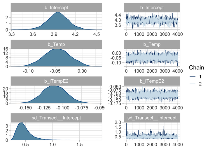
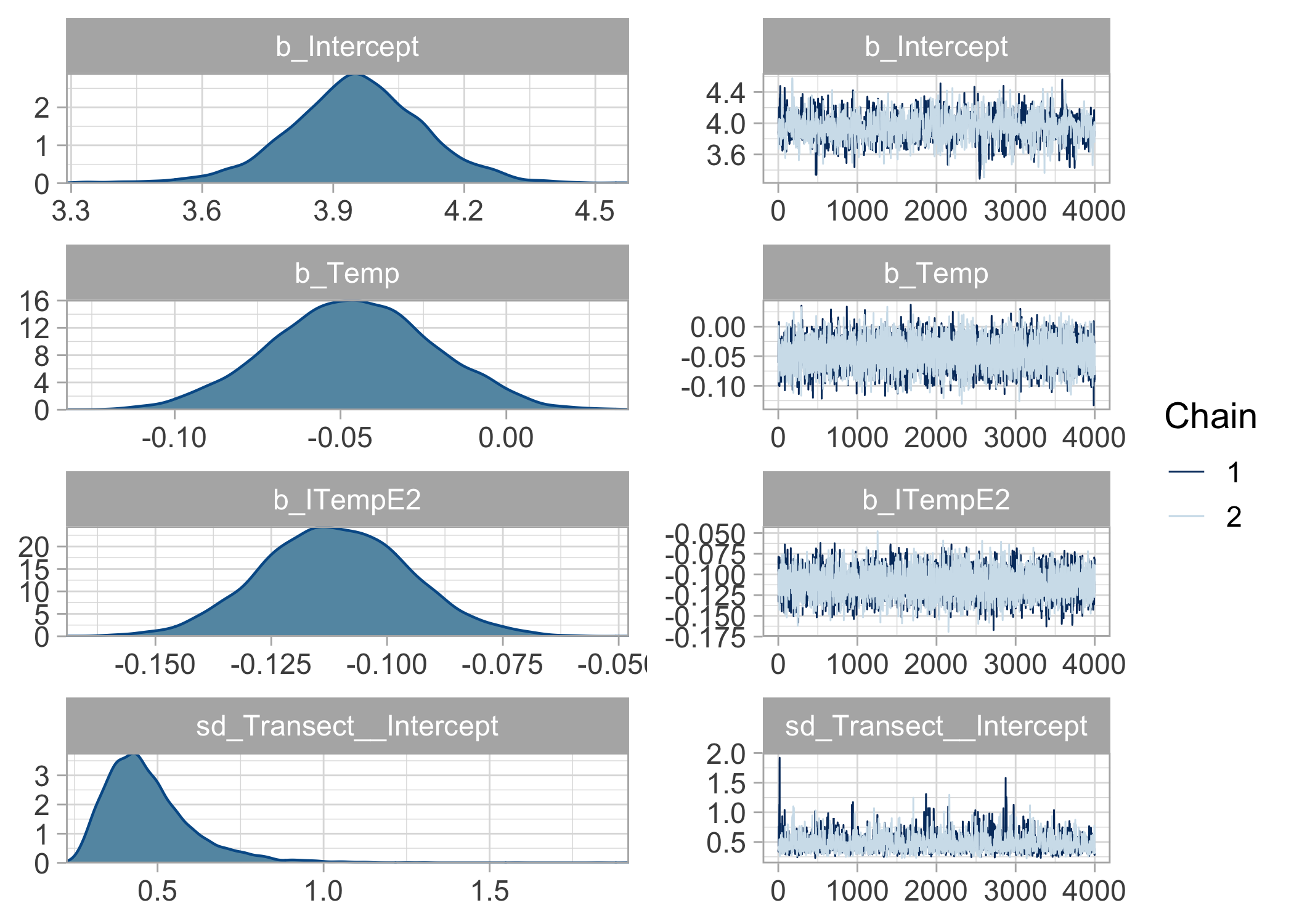
Visualize:
plot(bayes.brms)
We can assess the quality of fit of this model:
pp_check(bayes.brms, ndraws = 100, type = 'ecdf_overlay')
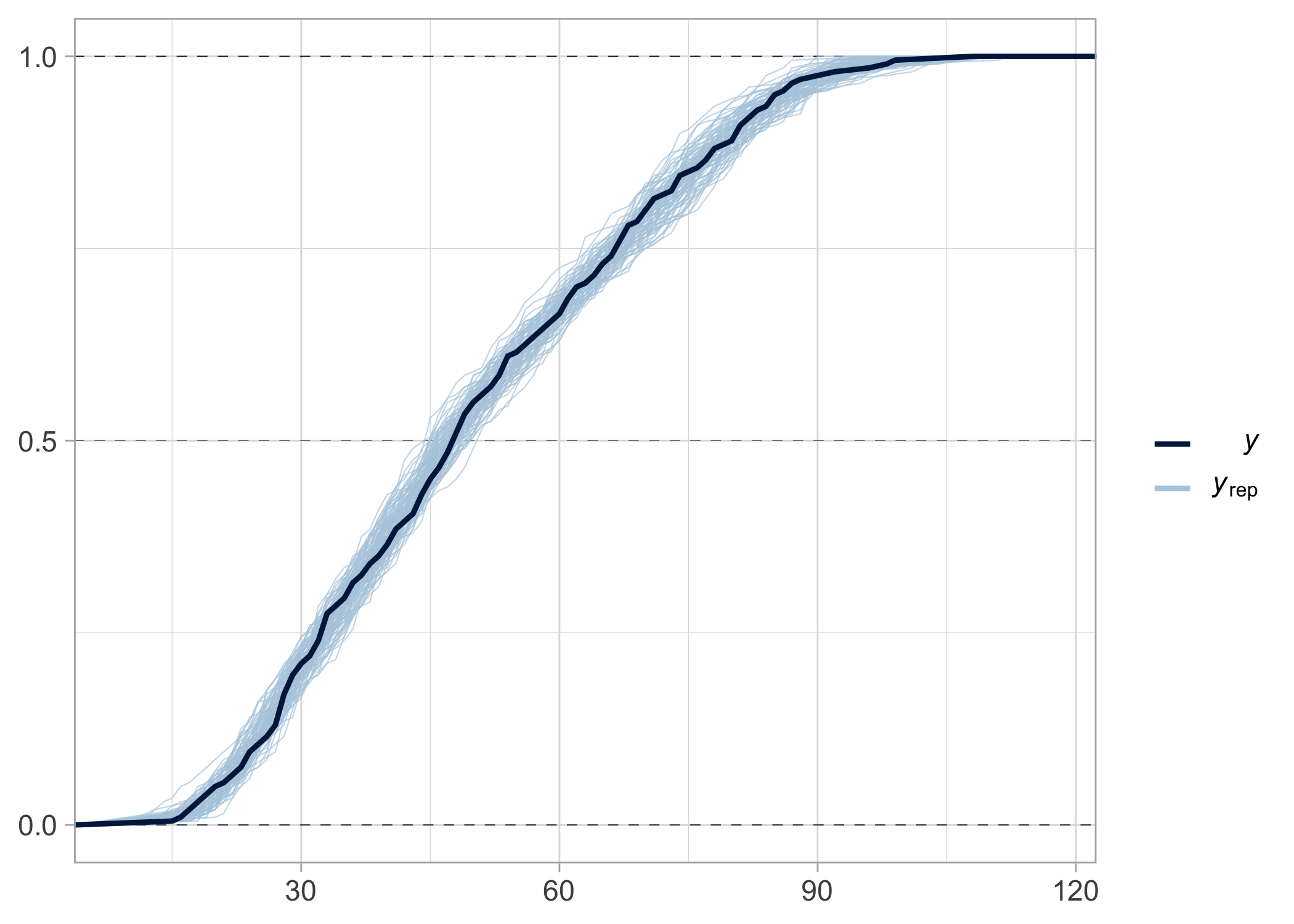
As expected, the fit is almost perfect because we simulated data from this very model.
What if we’d like to test the effect of temperature using WAIC?
We fit a model with no effect of temperature:
bayes.brms2 <- brm(Anemones ~ 1 + (1 | Transect),
                  data = data,
                  family = poisson("log"),
                  chains = 2, # nb of chains
                  iter = 5000, # nb of iterations, including burnin
                  warmup = 1000, # burnin
                  thin = 1)
## Running /Library/Frameworks/R.framework/Resources/bin/R CMD SHLIB foo.c
## clang -mmacosx-version-min=10.13 -I"/Library/Frameworks/R.framework/Resources/include" -DNDEBUG   -I"/Library/Frameworks/R.framework/Versions/4.1/Resources/library/Rcpp/include/"  -I"/Library/Frameworks/R.framework/Versions/4.1/Resources/library/RcppEigen/include/"  -I"/Library/Frameworks/R.framework/Versions/4.1/Resources/library/RcppEigen/include/unsupported"  -I"/Library/Frameworks/R.framework/Versions/4.1/Resources/library/BH/include" -I"/Library/Frameworks/R.framework/Versions/4.1/Resources/library/StanHeaders/include/src/"  -I"/Library/Frameworks/R.framework/Versions/4.1/Resources/library/StanHeaders/include/"  -I"/Library/Frameworks/R.framework/Versions/4.1/Resources/library/RcppParallel/include/"  -I"/Library/Frameworks/R.framework/Versions/4.1/Resources/library/rstan/include" -DEIGEN_NO_DEBUG  -DBOOST_DISABLE_ASSERTS  -DBOOST_PENDING_INTEGER_LOG2_HPP  -DSTAN_THREADS  -DBOOST_NO_AUTO_PTR  -include '/Library/Frameworks/R.framework/Versions/4.1/Resources/library/StanHeaders/include/stan/math/prim/mat/fun/Eigen.hpp'  -D_REENTRANT -DRCPP_PARALLEL_USE_TBB=1   -I/usr/local/include   -fPIC  -Wall -g -O2  -c foo.c -o foo.o
## In file included from <built-in>:1:
## In file included from /Library/Frameworks/R.framework/Versions/4.1/Resources/library/StanHeaders/include/stan/math/prim/mat/fun/Eigen.hpp:13:
## In file included from /Library/Frameworks/R.framework/Versions/4.1/Resources/library/RcppEigen/include/Eigen/Dense:1:
## In file included from /Library/Frameworks/R.framework/Versions/4.1/Resources/library/RcppEigen/include/Eigen/Core:88:
## /Library/Frameworks/R.framework/Versions/4.1/Resources/library/RcppEigen/include/Eigen/src/Core/util/Macros.h:628:1: error: unknown type name 'namespace'
## namespace Eigen {
## ^
## /Library/Frameworks/R.framework/Versions/4.1/Resources/library/RcppEigen/include/Eigen/src/Core/util/Macros.h:628:16: error: expected ';' after top level declarator
## namespace Eigen {
##                ^
##                ;
## In file included from <built-in>:1:
## In file included from /Library/Frameworks/R.framework/Versions/4.1/Resources/library/StanHeaders/include/stan/math/prim/mat/fun/Eigen.hpp:13:
## In file included from /Library/Frameworks/R.framework/Versions/4.1/Resources/library/RcppEigen/include/Eigen/Dense:1:
## /Library/Frameworks/R.framework/Versions/4.1/Resources/library/RcppEigen/include/Eigen/Core:96:10: fatal error: 'complex' file not found
## #include <complex>
##          ^~~~~~~~~
## 3 errors generated.
## make: *** [foo.o] Error 1
##
## SAMPLING FOR MODEL 'fd9804091450c044661531e89123d1dc' NOW (CHAIN 1).
## Chain 1:
## Chain 1: Gradient evaluation took 4.4e-05 seconds
## Chain 1: 1000 transitions using 10 leapfrog steps per transition would take 0.44 seconds.
## Chain 1: Adjust your expectations accordingly!
## Chain 1:
## Chain 1:
## Chain 1: Iteration:    1 / 5000 [  0%]  (Warmup)
## Chain 1: Iteration:  500 / 5000 [ 10%]  (Warmup)
## Chain 1: Iteration: 1000 / 5000 [ 20%]  (Warmup)
## Chain 1: Iteration: 1001 / 5000 [ 20%]  (Sampling)
## Chain 1: Iteration: 1500 / 5000 [ 30%]  (Sampling)
## Chain 1: Iteration: 2000 / 5000 [ 40%]  (Sampling)
## Chain 1: Iteration: 2500 / 5000 [ 50%]  (Sampling)
## Chain 1: Iteration: 3000 / 5000 [ 60%]  (Sampling)
## Chain 1: Iteration: 3500 / 5000 [ 70%]  (Sampling)
## Chain 1: Iteration: 4000 / 5000 [ 80%]  (Sampling)
## Chain 1: Iteration: 4500 / 5000 [ 90%]  (Sampling)
## Chain 1: Iteration: 5000 / 5000 [100%]  (Sampling)
## Chain 1:
## Chain 1:  Elapsed Time: 0.704799 seconds (Warm-up)
## Chain 1:                2.58736 seconds (Sampling)
## Chain 1:                3.29216 seconds (Total)
## Chain 1:
##
## SAMPLING FOR MODEL 'fd9804091450c044661531e89123d1dc' NOW (CHAIN 2).
## Chain 2:
## Chain 2: Gradient evaluation took 1.8e-05 seconds
## Chain 2: 1000 transitions using 10 leapfrog steps per transition would take 0.18 seconds.
## Chain 2: Adjust your expectations accordingly!
## Chain 2:
## Chain 2:
## Chain 2: Iteration:    1 / 5000 [  0%]  (Warmup)
## Chain 2: Iteration:  500 / 5000 [ 10%]  (Warmup)
## Chain 2: Iteration: 1000 / 5000 [ 20%]  (Warmup)
## Chain 2: Iteration: 1001 / 5000 [ 20%]  (Sampling)
## Chain 2: Iteration: 1500 / 5000 [ 30%]  (Sampling)
## Chain 2: Iteration: 2000 / 5000 [ 40%]  (Sampling)
## Chain 2: Iteration: 2500 / 5000 [ 50%]  (Sampling)
## Chain 2: Iteration: 3000 / 5000 [ 60%]  (Sampling)
## Chain 2: Iteration: 3500 / 5000 [ 70%]  (Sampling)
## Chain 2: Iteration: 4000 / 5000 [ 80%]  (Sampling)
## Chain 2: Iteration: 4500 / 5000 [ 90%]  (Sampling)
## Chain 2: Iteration: 5000 / 5000 [100%]  (Sampling)
## Chain 2:
## Chain 2:  Elapsed Time: 0.648008 seconds (Warm-up)
## Chain 2:                2.85026 seconds (Sampling)
## Chain 2:                3.49826 seconds (Total)
## Chain 2:
Then we compare both models, by ranking them with their WAIC or using ELPD:
(waic1 <- waic(bayes.brms)) # waic model w/ tempterature
##
## Computed from 8000 by 200 log-likelihood matrix
##
##           Estimate   SE
## elpd_waic   -668.2  9.8
## p_waic        11.0  1.1
## waic        1336.3 19.7
(waic2 <- waic(bayes.brms2)) # waic model wo/ tempterature
##
## Computed from 8000 by 200 log-likelihood matrix
##
##           Estimate   SE
## elpd_waic   -702.4 13.3
## p_waic        12.3  1.2
## waic        1404.9 26.5
##
## 2 (1.0%) p_waic estimates greater than 0.4. We recommend trying loo instead.
loo_compare(waic1, waic2)
##             elpd_diff se_diff
## bayes.brms    0.0       0.0
## bayes.brms2 -34.3       8.9
Conclusions
In all examples, you can check that i) there is little or no difference between Jags and brms numeric summaries of posterior distributions, and ii) maximum likelihood parameter estimates (glm(), lmer() and glmer() functions) and posterior means/medians are very close to each other.
In contrast to Jags, Nimble or Stan, you do not need to code the likelihood yourself in brms, as long as it is available in the package. You can have a look to a list of distributions with ?brms::brmsfamily, and there is also a possibility to define custom distributions with custom_family().
Note I haven’t covered diagnostics of convergence, more
here. You can also integrate brms outputs in a
tidy workflow with tidybayes, and use the ggplot() magic.
As usual, the code is on GitHub, visit https://github.com/oliviergimenez/fit-glmm-with-brms.
Now I guess it’s up to the students to pick their favorite Bayesian tool.