Here I illustrate how to train a CNN with Keras in R to predict from patients’ CT scans those who will develop severe illness from Covid.

Motivation

Michael Blum tweeted about the STOIC2021 - COVID-19 AI challenge. The main goal of this challenge is to predict from the patients’ CT scans who will develop severe illness from Covid.

Given my recent interest in machine learning, this challenge peaked my interest. Although Python is the machine learning lingua franca, it is possible to train a convolutional neural network (CNN) in R and perform (binary) image classification.

Here, I will use an R interface to Keras that allows training neural networks. Note that the dataset shared for the challenge is big, like 280Go big, and it took me a day to download it. For the sake of illustration, I will use a similar but much lighter dataset from a Kaggle repository https://www.kaggle.com/plameneduardo/sarscov2-ctscan-dataset.

The code is available on GitHub as usual https://github.com/oliviergimenez/bin-image-classif.

First things first, load the packages we will need.

library(tidyverse)
theme_set(theme_light())
library(keras)

Read in and process data

We will need a function to process images, I’m stealing that one written by Spencer Palladino.

process_pix <- function(lsf) {
  img <- lapply(lsf, image_load, grayscale = TRUE) # grayscale the image
  arr <- lapply(img, image_to_array) # turns it into an array
  arr_resized <- lapply(arr, image_array_resize, 
                        height = 100, 
                        width = 100) # resize
  arr_normalized <- normalize(arr_resized, axis = 1) #normalize to make small numbers 
  return(arr_normalized)
}

Now let’s process images for patients with Covid, and do some reshaping. Idem with images for patients without Covid.

# with covid
lsf <- list.files("dat/COVID/", full.names = TRUE) 
covid <- process_pix(lsf)
covid <- covid[,,,1] # get rid of last dim
covid_reshaped <- array_reshape(covid, c(nrow(covid), 100*100))
# without covid
lsf <- list.files("dat/non-COVID/", full.names = TRUE) 
ncovid <- process_pix(lsf)
ncovid <- ncovid[,,,1] # get rid of last dim
ncovid_reshaped <- array_reshape(ncovid, c(nrow(ncovid), 100*100))

We have 1252 CT scans of patients with Covid, and 1229 without.

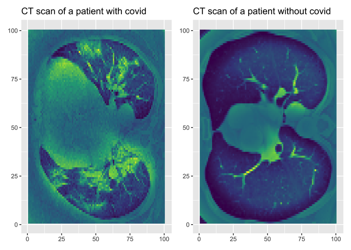
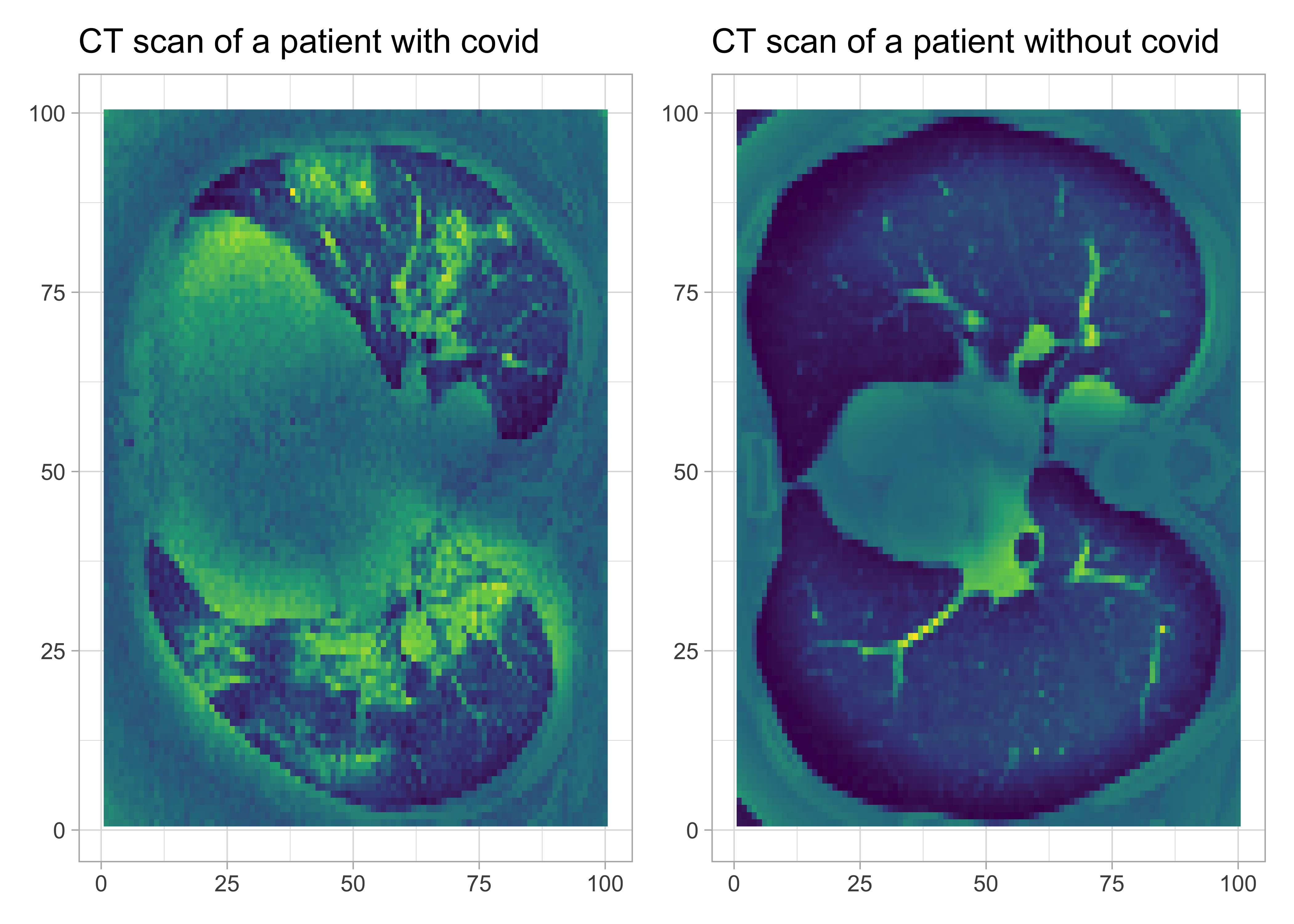
Let’s visualise these scans. Let’s pick a patient with Covid, and another one without.

scancovid <- reshape2::melt(covid[10,,])
plotcovid <- scancovid %>%
  ggplot() +
  aes(x = Var1, y = Var2, fill = value) + 
  geom_raster() +
  labs(x = NULL, y = NULL, title = "CT scan of a patient with covid") + 
  scale_fill_viridis_c() + 
  theme(legend.position = "none")

scanncovid <- reshape2::melt(ncovid[10,,])
plotncovid <- scanncovid %>%
  ggplot() +
  aes(x = Var1, y = Var2, fill = value) + 
  geom_raster() +
  labs(x = NULL, y = NULL, title = "CT scan of a patient without covid") + 
  scale_fill_viridis_c() + 
  theme(legend.position = "none")

library(patchwork)
plotcovid + plotncovid

Put altogether and shuffle.

df <- rbind(cbind(covid_reshaped, 1), # 1 = covid
            cbind(ncovid_reshaped, 0)) # 0 = no covid
set.seed(1234)
shuffle <- sample(nrow(df), replace = F)
df <- df[shuffle, ]

Sounds great. We have everything we need to start training a convolutional neural network model.

Convolutional neural network (CNN)

Let’s build our training and testing datasets using a 80/20 split.

set.seed(2022)
split <- sample(2, nrow(df), replace = T, prob = c(0.8, 0.2))
train <- df[split == 1,]
test <- df[split == 2,]
train_target <- df[split == 1, 10001] # label in training dataset
test_target <- df[split == 2, 10001] # label in testing dataset

Now build our model. I use three layers (layer_dense() function) that I put one after the other with piping. I also use regularization (layer_dropout() function) to avoid overfitting.

model <- keras_model_sequential() %>%
  layer_dense(units = 512, activation = "relu") %>% 
  layer_dropout(0.4) %>%
  layer_dense(units = 256, activation = "relu") %>%
  layer_dropout(0.3) %>%
  layer_dense(units = 128, activation = "relu") %>%
  layer_dropout(0.2) %>%
  layer_dense(units = 2, activation = 'softmax')

Compile the model with defaults specific to binary classification.

model %>%
  compile(optimizer = 'adam',
          loss = 'binary_crossentropy', 
          metrics = c('accuracy'))

We use one-hot encoding (to_categorical() function) aka dummy coding in statistics.

train_label <- to_categorical(train_target)
test_label <- to_categorical(test_target)

Now let’s fit our model to the training dataset.

fit_covid <- model %>%
  fit(x = train,
      y = train_label, 
      epochs = 25,
      batch_size = 512, # try also 128 and 256
      verbose = 2,
      validation_split = 0.2)

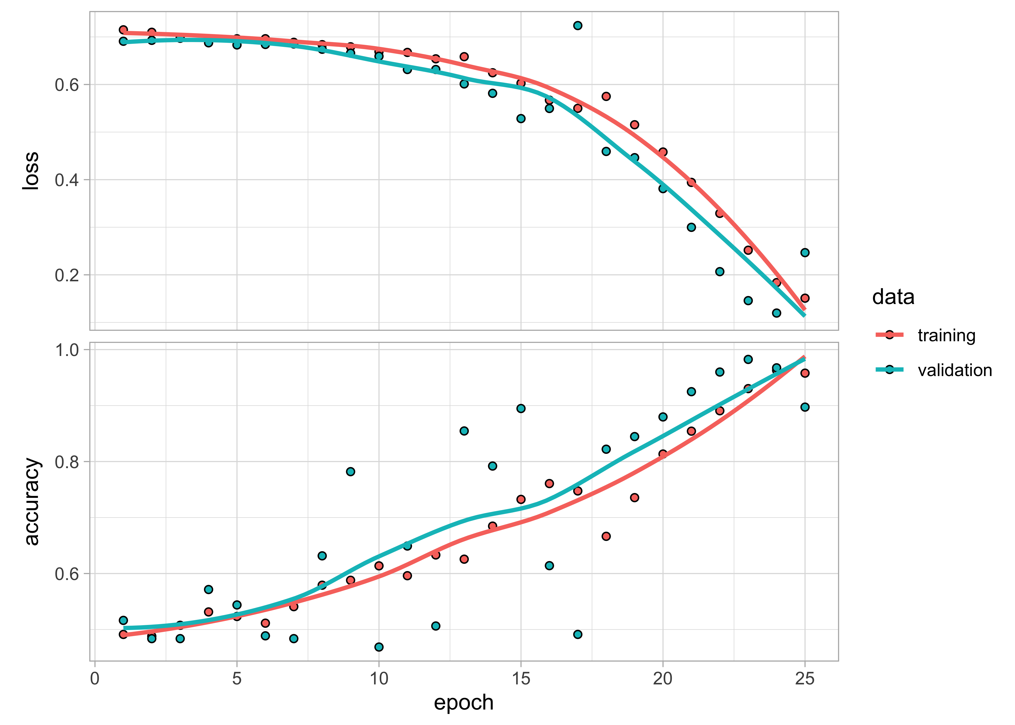
A quick visualization of the performances shows that the algorithm is doing not too bad. No over/under-fitting. Accuracy and loss are fine.

plot(fit_covid)

What about the performances on the testing dataset?

model %>%
  evaluate(test, test_label)

##       loss   accuracy 
## 0.02048795 0.99795920

Let’s do some predictions on the testing dataset, and compare with ground truth.

predictedclasses <- model %>%
  predict_classes(test)
table(Prediction = predictedclasses, 
      Actual = test_target)

##           Actual
## Prediction   0   1
##          0 243   0
##          1   1 246

Pretty cool. Only one healthy patient is misclassified as being sick. Let’s save our model for further use.

save_model_tf(model, "model/covidmodel") # save the model

I’m happy with these results. In general however, we need to find ways to improve the performances. Check out some tips here with examples implemented in Keras with R there.