Simulating data with JAGS

Here, I illustrate the possibility to use `JAGS` to simulate data with two examples that might be of interest to population ecologists: first a linear regression, second a Cormack-Jolly-Seber capture-recapture model to estimate animal survival (formulated as a state-space model). The code is available from [GitHub](https://github.com/oliviergimenez/simul_with_jags).

Recently, I have been struggling with simulating data from complex hierarchical models. After several unsuccessful attempts in R, I remembered the good old times when I was using WinBUGS (more than 10 years already!) and the possibility to simulate data with it. I’m using JAGS now, and a quick search in Google with ‘simulating data with jags’ led me to a complex example and a simple example.

Simulating data with JAGS is convenient because you can use (almost) the same code for simulation and inference, and you can carry out simulation studies (bias, precision, interval coverage) in the same environment (namely JAGS).

Linear regression example

We first load the packages we need for this tutorial:

library(R2jags)
library(runjags)
library(mcmcplots)

Then straight to the point, let’s generate data from a linear regression model. The trick is to use a data block, have the simplest model block you could think of and pass the parameters as if they were data. Note that it’d be possible to use only a model block, see comment here.

txtstring <- '
data{
# Likelihood:
for (i in 1:N){
y[i] ~ dnorm(mu[i], tau) # tau is precision (1 / variance)
mu[i] <- alpha + beta * x[i]
}
}
model{
fake <- 0
}
'

Here, alpha and beta are the intercept and slope, tau the precision or the inverse of the variance, y the response variable and x the explanatory variable.

We pick some values for the model parameters that we will use as data:

# parameters for simulations 
N = 30 # nb of observations
x <- 1:N # predictor
alpha = 0.5 # intercept
beta = 1 # slope
sigma <- .1 # residual sd
tau <- 1/(sigma*sigma) # precision
# parameters are treated as data for the simulation step
data<-list(N=N,x=x,alpha=alpha,beta=beta,tau=tau)

Now call JAGS; note that we monitor the response variable instead of parameters as we would do when conducting standard inference:

# run jags
out <- run.jags(txtstring, data = data,monitor=c("y"),sample=1, n.chains=1, summarise=FALSE)

## Compiling rjags model...
## Calling the simulation using the rjags method...
## Note: the model did not require adaptation
## Burning in the model for 4000 iterations...
## Running the model for 1 iterations...
## Simulation complete
## Finished running the simulation

The output is a bit messy and needs to be formatted appropriately:

# reformat the outputs
Simulated <- coda::as.mcmc(out)
Simulated

## Markov Chain Monte Carlo (MCMC) output:
## Start = 5001 
## End = 5001 
## Thinning interval = 1 
##          y[1]    y[2]    y[3]     y[4]     y[5]     y[6]     y[7]     y[8]
## 5001 1.288399 2.52408 3.61516 4.583587 5.600675 6.566052 7.593407 8.457497
##         y[9]    y[10]   y[11]    y[12]    y[13]    y[14]    y[15]    y[16]
## 5001 9.70847 10.38035 11.5105 12.55048 13.49143 14.46356 15.45641 16.56148
##         y[17]    y[18]    y[19]    y[20]    y[21]   y[22]    y[23]
## 5001 17.50935 18.51501 19.66197 20.49477 21.57079 22.6199 23.48232
##         y[24]    y[25]    y[26]    y[27]    y[28]    y[29]    y[30]
## 5001 24.57923 25.47368 26.33674 27.46525 28.35525 29.60279 30.42952

dim(Simulated)

## [1]  1 30

dat = as.vector(Simulated)
dat

##  [1]  1.288399  2.524080  3.615160  4.583587  5.600675  6.566052  7.593407
##  [8]  8.457497  9.708470 10.380351 11.510500 12.550482 13.491435 14.463564
## [15] 15.456410 16.561483 17.509350 18.515005 19.661969 20.494767 21.570790
## [22] 22.619899 23.482317 24.579228 25.473676 26.336736 27.465251 28.355248
## [29] 29.602791 30.429517

Now let’s fit the model we used to simulate to the data we just generated. I won’t go into the details and assume that the reader is familiar with JAGS and linear regression.

# specify model in BUGS language
model <- 	
paste("	
model {
# Likelihood:
for (i in 1:N){
y[i] ~ dnorm(mu[i], tau) # tau is precision (1 / variance)
mu[i] <- alpha + beta * x[i]
}
# Priors:
alpha ~ dnorm(0, 0.01) # intercept
beta ~ dnorm(0, 0.01) # slope
sigma ~ dunif(0, 100) # standard deviation
tau <- 1 / (sigma * sigma) 
}
")
writeLines(model,"lin_reg.jags")	

# data
jags.data <- list(y = dat, N = length(dat), x = x)

# initial values
inits <- function(){list(alpha = rnorm(1), beta = rnorm(1), sigma = runif(1,0,10))}  

# parameters monitored
parameters <- c("alpha", "beta", "sigma")

# MCMC settings
ni <- 10000
nt <- 6
nb <- 5000
nc <- 2

# call JAGS from R
res <- jags(jags.data, inits, parameters, "lin_reg.jags", n.chains = nc, n.thin = nt, n.iter = ni, n.burnin = nb, working.directory = getwd())

## module glm loaded

## Compiling model graph
##    Resolving undeclared variables
##    Allocating nodes
## Graph information:
##    Observed stochastic nodes: 30
##    Unobserved stochastic nodes: 3
##    Total graph size: 130
## 
## Initializing model

Let’s have a look to the results and compare with the parameters we used to simulate the data (see above):

# summarize posteriors
print(res, digits = 3)

## Inference for Bugs model at "lin_reg.jags", fit using jags,
##  2 chains, each with 10000 iterations (first 5000 discarded), n.thin = 6
##  n.sims = 1668 iterations saved
##          mu.vect sd.vect    2.5%     25%     50%     75%   97.5%  Rhat
## alpha      0.544   0.038   0.469   0.518   0.545   0.570   0.617 1.000
## beta       0.998   0.002   0.994   0.997   0.998   1.000   1.003 1.001
## sigma      0.102   0.015   0.078   0.091   0.100   0.110   0.138 1.002
## deviance -53.810   2.724 -56.867 -55.808 -54.516 -52.641 -46.676 1.001
##          n.eff
## alpha     1700
## beta      1700
## sigma      780
## deviance  1700
## 
## For each parameter, n.eff is a crude measure of effective sample size,
## and Rhat is the potential scale reduction factor (at convergence, Rhat=1).
## 
## DIC info (using the rule, pD = var(deviance)/2)
## pD = 3.7 and DIC = -50.1
## DIC is an estimate of expected predictive error (lower deviance is better).

Pretty close!

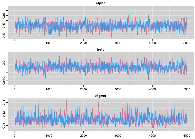
Check convergence:

# trace plots
traplot(res,c("alpha", "beta", "sigma"))

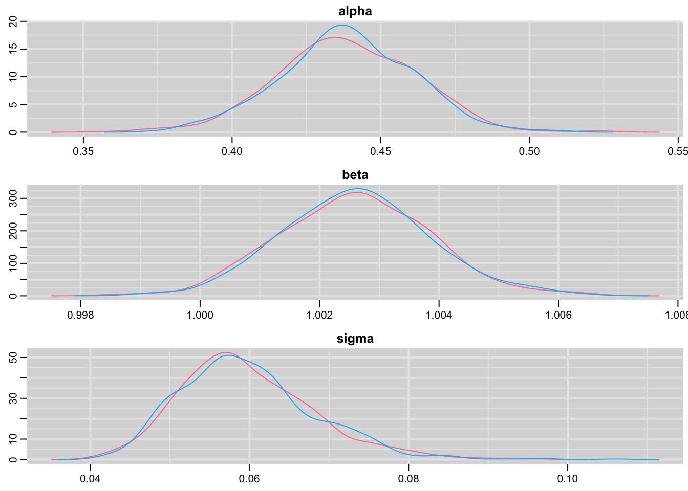
Plot the posterior distribution of the regression parameters and residual standard deviation:

# posterior distributions
denplot(res,c("alpha", "beta", "sigma"))

Capture-recapture example

I now illustrate the use of JAGS to simulate data from a Cormack-Jolly-Seber model with constant survival and recapture probabilities. I assume that the reader is familiar with this model and its formulation as a state-space model.

Let’s simulate!

txtstring <- '
data{
# Constant survival and recapture probabilities
for (i in 1:nind){
   for (t in f[i]:(n.occasions-1)){
      phi[i,t] <- mean.phi
      p[i,t] <- mean.p
      } #t
   } #i
# Likelihood 
for (i in 1:nind){
   # Define latent state and obs at first capture
   z[i,f[i]] <- 1
   mu2[i,1] <- 1 * z[i,f[i]] # detection is 1 at first capture ("conditional on first capture")
   y[i,1] ~ dbern(mu2[i,1])
   # then deal w/ subsequent occasions
   for (t in (f[i]+1):n.occasions){
      # State process
      z[i,t] ~ dbern(mu1[i,t])
      mu1[i,t] <- phi[i,t-1] * z[i,t-1]
      # Observation process
      y[i,t] ~ dbern(mu2[i,t])
      mu2[i,t] <- p[i,t-1] * z[i,t]
      } #t
   } #i
}
model{
fake <- 0
}
'

Let’s pick some values for parameters and store them in a data list:

# parameter for simulations 
n.occasions = 10 # nb of occasions
nind = 100 # nb of individuals
mean.phi <- 0.8 # survival
mean.p <- 0.6 # recapture
f = rep(1,nind) # date of first capture
data<-list(n.occasions = n.occasions, mean.phi = mean.phi, mean.p = mean.p, f = f, nind = nind)

Now run JAGS:

out <- run.jags(txtstring, data = data,monitor=c("y"),sample=1, n.chains=1, summarise=FALSE)

## Compiling rjags model...
## Calling the simulation using the rjags method...
## Note: the model did not require adaptation
## Burning in the model for 4000 iterations...
## Running the model for 1 iterations...
## Simulation complete
## Finished running the simulation

Format the output:

Simulated <- coda::as.mcmc(out)
dim(Simulated)

## [1]    1 1000

dat = matrix(Simulated,nrow=nind)
head(dat)

##      [,1] [,2] [,3] [,4] [,5] [,6] [,7] [,8] [,9] [,10]
## [1,]    1    1    0    0    0    0    0    0    0     0
## [2,]    1    1    1    1    0    0    0    0    0     0
## [3,]    1    0    0    0    0    0    0    0    0     0
## [4,]    1    0    0    0    0    0    0    0    0     0
## [5,]    1    0    0    0    0    0    0    0    0     0
## [6,]    1    1    1    1    0    0    1    0    1     1

Here I monitored only the detections and non-detections, but it is also possible to get the simulated values for the states, i.e. whether an individual is alive or dead at each occasion. You just need to amend the call to JAGS with monitor=c("y","x") and to amend the output accordingly.

Now we fit a Cormack-Jolly-Seber model to the data we’ve just simulated, assuming constant parameters:

model <- 	
paste("	
model {
# Priors and constraints
for (i in 1:nind){
   for (t in f[i]:(n.occasions-1)){
      phi[i,t] <- mean.phi
      p[i,t] <- mean.p
      } #t
   } #i
mean.phi ~ dunif(0, 1)         # Prior for mean survival
mean.p ~ dunif(0, 1)           # Prior for mean recapture
# Likelihood 
for (i in 1:nind){
   # Define latent state at first capture
   z[i,f[i]] <- 1
   for (t in (f[i]+1):n.occasions){
      # State process
      z[i,t] ~ dbern(mu1[i,t])
      mu1[i,t] <- phi[i,t-1] * z[i,t-1]
      # Observation process
      y[i,t] ~ dbern(mu2[i,t])
      mu2[i,t] <- p[i,t-1] * z[i,t]
      } #t
   } #i
}
")
writeLines(model,"cjs.jags")	

Prepare the data:

# vector with occasion of marking
get.first <- function(x) min(which(x!=0))
f <- apply(dat, 1, get.first)
# data
jags.data <- list(y = dat, f = f, nind = dim(dat)[1], n.occasions = dim(dat)[2])

# Initial values
known.state.cjs <- function(ch){
   state <- ch
   for (i in 1:dim(ch)[1]){
      n1 <- min(which(ch[i,]==1))
      n2 <- max(which(ch[i,]==1))
      state[i,n1:n2] <- 1
      state[i,n1] <- NA
      }
   state[state==0] <- NA
   return(state)
   }
inits <- function(){list(mean.phi = runif(1, 0, 1), mean.p = runif(1, 0, 1), z = known.state.cjs(dat))}

We’d like to carry out inference about survival and recapture probabilities:

parameters <- c("mean.phi", "mean.p")

Standard MCMC settings:

ni <- 10000
nt <- 6
nb <- 5000
nc <- 2

Ready to run JAGS!

# Call JAGS from R (BRT 1 min)
cjs <- jags(jags.data, inits, parameters, "cjs.jags", n.chains = nc, n.thin = nt, n.iter = ni, n.burnin = nb, working.directory = getwd())

## Compiling model graph
##    Resolving undeclared variables
##    Allocating nodes
## Graph information:
##    Observed stochastic nodes: 900
##    Unobserved stochastic nodes: 902
##    Total graph size: 3707
## 
## Initializing model

Summarize posteriors and compare to the values we used to simulate the data:

print(cjs, digits = 3)

## Inference for Bugs model at "cjs.jags", fit using jags,
##  2 chains, each with 10000 iterations (first 5000 discarded), n.thin = 6
##  n.sims = 1668 iterations saved
##          mu.vect sd.vect    2.5%     25%     50%     75%   97.5%  Rhat
## mean.p     0.596   0.033   0.531   0.574   0.597   0.618   0.660 1.000
## mean.phi   0.784   0.021   0.742   0.770   0.785   0.799   0.824 1.001
## deviance 440.611  18.374 408.121 427.569 438.662 452.512 479.608 1.001
##          n.eff
## mean.p    1700
## mean.phi  1700
## deviance  1700
## 
## For each parameter, n.eff is a crude measure of effective sample size,
## and Rhat is the potential scale reduction factor (at convergence, Rhat=1).
## 
## DIC info (using the rule, pD = var(deviance)/2)
## pD = 168.9 and DIC = 609.5
## DIC is an estimate of expected predictive error (lower deviance is better).

Again pretty close!

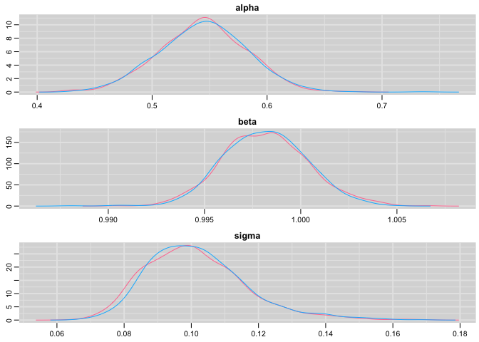
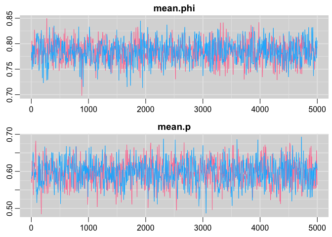
Trace plots

traplot(cjs,c("mean.phi", "mean.p"))

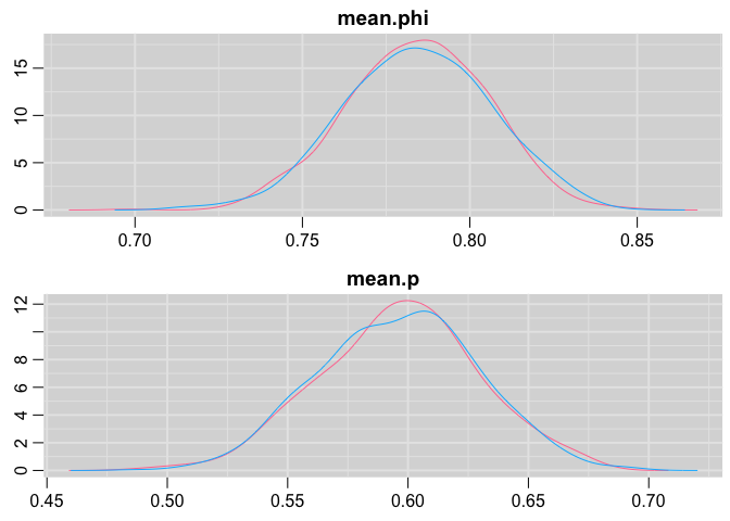
Posterior distribution plots:

denplot(cjs,c("mean.phi", "mean.p"))