Scientific research is all about networking

I read this awesome post (in French) by Baptiste Coulmont, professor in sociology, who explored the French academic network in sociology. Coulmont used the composition of PhD commitees to determine academic links between colleagues. The approach very appealing because it uses public data available from the website these.fr. Here, I used Coulmont’s R code to produce the French academic network in ecology. This was a nice opportunity to illustrate how to work in the tidyverse and to do some web scraping using the rvest package.

Get the data

Load the packages we need:

library(RCurl)
library(tidyverse)
library(lubridate)
library(scales)
library(hrbrthemes)
library(data.table)
# devtools::install_github("privefl/bigreadr")
library(bigreadr)

We now prepare the URL requests. The total number of PhDs is around 88000 on the period 2015-2018. Because the website uses slices of 1000 on each page, we proceed in sequence:

i <- 1:88
i <- i*1000
URL <-paste0("http://www.theses.fr/?q=&fq=dateSoutenance:[2015-01-01T23:59:59Z%2BTO%2B2018-12-31T23:59:59Z]&checkedfacets=&start=",i,"&sort=none&status=&access=&prevision=&filtrepersonne=&zone1=titreRAs&val1=&op1=AND&zone2=auteurs&val2=&op2=AND&zone3=etabSoutenances&val3=&zone4=dateSoutenance&val4a=&val4b=&type=&lng=&checkedfacets=&format=csv")

Alternatively, the search can be done by hand directly from the theses.fr website. [François-Xavier Coudert] ( https://www.coudert.name/) also provides the search results for the 2015-2018 period.

We proceed with the requests, and store everything in a csv file:

j <- 1
SERP <- 1
for(j in 1:length(URL)){ # loop over the slices
  SERP[j] <- getURL(URL[j])
  write.csv(SERP,"SERP_2.csv",append=F)
}
rm(SERP,i,j,URL)

We keep only the PhDs in the field (Discipline) of ecology. This is basically the only change I have made to Coulmont’s neat code.

theses <- read.csv("SERP_2.csv",sep=";",quote="",skip=1,stringsAsFactors = F)
#theses %>% 
#  pull(X..Discipline..) %>% 
#  unique()

ecology <- theses %>% filter(grepl("ecologie",X..Discipline..,ignore.case=T)) %>% # keep PhDs with Displine == ecologie
  filter(X..Date.de.soutenance..!="") %>% # remove PhDs with missing dates of defense
  filter(X..Statut..=="soutenue") # keep only PhDs that have been defended

We now have the id of all PhDs in ecology defended during the period 2015-2018. We will use the id to get the composition of all PhD commitees. Getting this composition requires scraping the web page of each PhD, and to get the ID of each PhD. For doing so, we use the rvest package (see the excellent posts by Maëlle Salmon for examples).

library(rvest)
identifiants <- ecology$X..Identifiant.de.la.these.. # get PhD ids
reseau_total <- data_frame(noms_jury="",
                           liens_jury="",
                           these="",
                           directeurs="",
                           liens_directeurs="")

for (i in 1:length(identifiants)) {
  
  # get info on current PhD
  data_theses_eco <- read_html( paste0("http://www.theses.fr/",identifiants[i]) ) 

  # get name PhD supervisor for 
  directeurs <- bind_cols(
    directeurs = data_theses_eco  %>%
      html_nodes("div .donnees-ombre p") %>%
      .[[1]] %>%
      html_nodes("a") %>%
      html_text()
    ,
    liens_directeurs = data_theses_eco  %>%
      html_nodes("div .donnees-ombre p") %>%
      .[[1]] %>%
      html_nodes("a") %>%
      html_attr(name="href")
  ) %>% mutate(  these = identifiants[i] )
  
  # get names of people in commitees
    jury <- bind_cols( 
    noms_jury = data_theses_eco %>%
      html_nodes("div .donnees p a") %>%
      html_text()
    ,
    liens_jury = data_theses_eco %>%
      html_nodes("div .donnees p a") %>%
      html_attr(name="href")
  ) %>% mutate(  these = identifiants[i] )
    
  # put all together
    reseau <- jury %>% left_join(directeurs,by="these") 
    reseau_total <- bind_rows(reseau_total,reseau)
}

Build the network

Load the packages we need, and the data we got at the previous step:

library(igraph)
library(ggraph)
library(ggrepel)
load('reseau_total.RData')

Coulmont defined a weighted link between two colleagues i and j as follows: 3 if i and j are both supervisors, 2 if i is a supervisor and j a PhD commitee member and 1 if both i and j are PhD commitee members. A colleague may accumulate several weights.

directions_theses <- reseau_total %>% 
  select(these,directeurs) %>% 
  unique() %>% 
  group_by(these) %>% 
  mutate(N=n()) %>%
  filter(N==2) %>% # keep co-supervision w/ 2 supervisors 
  mutate(rang=rank(directeurs)) %>% 
  spread(key=rang,value=directeurs) %>% 
  ungroup() %>% 
  select(nom1=`1`,nom2=`2`) %>% 
  mutate(poids=3)

directions_jury <- reseau_total %>% 
  select(nom1=noms_jury,nom2=directeurs) %>% 
  filter( nom1 != "") %>%
  mutate(poids=2) %>%
  group_by(nom1,nom2) %>% 
  summarize(poids=sum(poids))

jury_jury <- reseau_total %>% 
  select(noms_jury,these) %>% 
  unique() %>% 
  filter(noms_jury!="")

g_j <-  graph_from_data_frame(jury_jury,directed=F)
V(g_j)$type <- V(g_j)$name %in% jury_jury$noms_jury
g_j_1 <- bipartite_projection(g_j,which="true")
jurys <- as_long_data_frame(g_j_1) %>%
  select(nom1=`ver[el[, 1], ]`, nom2=`ver2[el[, 2], ]`, poids=weight)

reseau_petit <- bind_rows(directions_theses,directions_jury,jurys) %>%
  group_by(nom1,nom2) %>% 
  summarize(poids=sum(poids)) # data.frame from which the network will be created

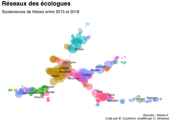
Each node in the network has a size proportional to its betweenness score. We also determine communities using the walktrap algorithm that will be colored differently. The width of an edge is proportional to the strength of the link between the two corresponding nodes.

g <- graph_from_data_frame(reseau_petit, directed=F) # create network from data.frame
g <- simplify(g,edge.attr.comb = sum)
V(g)$degres <-  degree(g)
V(g)$label <- gsub("^\\S+\\s+(.+)$","\\1",V(g)$name)
V(g)$communaute <- as.character(cluster_walktrap(g, steps=15)$membership) # determine communities
V(g)$closeness <- (5*closeness(g))^10
V(g)$btwns <- betweenness(g) # network metric betweeness
V(g)$eigen_centr <- eigen_centrality(g)$vector
g <- delete_edges(g, which(E(g)$poids<5) ) # delete edges with weight <= 4
V(g)$cluster_number <- clusters(g)$membership # to which community you belong
g <- induced_subgraph(g, V(g)$cluster_number== which( max(clusters(g)$csize) == clusters(g)$csize) )
E(g)$weight <- 1/E(g)$poids # width of edge proportional to weight
V(g)$label <- ifelse(V(g)$degres<20,"",V(g)$label) # do not display all names

Plot the network

We now plot the network. For clarity, we only indicate the names of colleagues who were part of several phD commitees.

ggraph(g,layout="igraph",algorithm="fr") + 
  geom_edge_link(aes(width=.1*poids), alpha=.1, 
                 end_cap = circle(5, 'mm'), 
                 start_cap = circle(5, 'mm')) +
  geom_node_point(aes(size=eigen_centr), color="white",alpha=1) +
  geom_node_point(aes(color=communaute,size=eigen_centr), alpha=.5) +
  scale_size_area(max_size = 20) +
  geom_node_text(aes(label=label),size=3,repel=T,box.padding = 0.15) +
  labs(title="Réseaux des écologues",
       subtitle="Soutenances de thèses entre 2015 et 2018",
       caption="Sources : theses.fr \n Code par B. Coulmont, modifié par O. Gimenez") +
  theme_graph(foreground = 'white', fg_text_colour = 'white',
              base_family = "Helvetica") +
  theme(legend.position="none",
        text=element_text(size=16,family="Helvetica"),
        plot.margin = unit(c(0.2, 0.2, 0.2, 0.2), units="line"))

# save
ggsave(filename = "ecology_network.pdf",width=30,height = 20)

I played around the defaults Coulmont used to build and plot the network. It helps in getting a better understanding of the network and the links between colleagues working in ecology. Overall, I indeed feel very much connected to my colleagues in Montpellier, Lyon and Grenoble. I should probably go out of my comfort zone and interact even more with my colleagues from La Rochelle, Marseille and Aix-en-Provence 😃

As always, data and code are available from GitHub.