Motivation
Below are some notes I have taken on David Robinson’s screencasts, with tips and tricks I use for my own R peregrinations in the Tidyverse framework. Hopefully, these notes will be useful to others. I assume you know the basics of the Tidyverse. If not, check out the quick and dirty introduction to the Tidyverse I wrote some time ago.
It took me some time to fully transition from base R to the Tidyverse. I really clicked when I started watching screencasts by David Robinson on his Youtube channel.
Each week, he goes live for an hour or so, and does exploratory analyses in R with data he has never seen before (!). The data come from the #TidyTuesday project brought to us by the R for Data Science Online Learning Community. This is an awesome initiative, check out the beautiful #tidytuesday visualisations on Twitter.
David Robinson shares the #RStats code he writes during his screencasts, and provides annotations for us to grasp at once what the screencast is about, and what the main steps of the analyses are (including the R functions he uses).
Below are my personal notes, with an obvious bias towards the tricks I find useful for my own work. Check out David Robinson’s talk Ten Tremendous Tricks for Tidyverse. You will also be interested in Emily Robinson’s talk The Lesser Known Stars of the Tidyverse.
Let’s get to it. First data wrangling, second data visualisation. I will use some of the awesome illustrations by Allison Horst throughout, check out her work here.
Setting the scene

Load the tidyverse suite of packages:
library(tidyverse)
## ── Attaching packages ─────────────────────────────────────── tidyverse 1.3.1 ──
## ✔ ggplot2 3.3.5          ✔ purrr   0.3.4.9000
## ✔ tibble  3.1.6          ✔ dplyr   1.0.7
## ✔ tidyr   1.1.4          ✔ stringr 1.4.0
## ✔ readr   2.0.0          ✔ forcats 0.5.1
## ── Conflicts ────────────────────────────────────────── tidyverse_conflicts() ──
## ✖ dplyr::filter() masks stats::filter()
## ✖ dplyr::lag()    masks stats::lag()
By the way, if you need to explore the functions of a package, a trick is to use the autocompletion in RStudio. Just type in ?package_name:: and you should see the functions of the package_name package in a pull-down menu.
Now set the theme you like for data visualisation with ggplot2:
theme_set(theme_light())
For illustration, I will use the starwars dataset that comes with the tidyverse collection of packages:
data("starwars")
starwars_raw <- starwars
Data wrangling
Inspect the data
Use the viewer View() to inspect your data:
starwars_raw %>%
  View()
The tibble format is great to double check the format of your columns:
starwars_raw
## # A tibble: 87 × 14
##    name     height  mass hair_color skin_color eye_color birth_year sex   gender
##    <chr>     <int> <dbl> <chr>      <chr>      <chr>          <dbl> <chr> <chr>
##  1 Luke Sk…    172    77 blond      fair       blue            19   male  mascu…
##  2 C-3PO       167    75 <NA>       gold       yellow         112   none  mascu…
##  3 R2-D2        96    32 <NA>       white, bl… red             33   none  mascu…
##  4 Darth V…    202   136 none       white      yellow          41.9 male  mascu…
##  5 Leia Or…    150    49 brown      light      brown           19   fema… femin…
##  6 Owen La…    178   120 brown, gr… light      blue            52   male  mascu…
##  7 Beru Wh…    165    75 brown      light      blue            47   fema… femin…
##  8 R5-D4        97    32 <NA>       white, red red             NA   none  mascu…
##  9 Biggs D…    183    84 black      light      brown           24   male  mascu…
## 10 Obi-Wan…    182    77 auburn, w… fair       blue-gray       57   male  mascu…
## # … with 77 more rows, and 5 more variables: homeworld <chr>, species <chr>,
## #   films <list>, vehicles <list>, starships <list>
chr, int, dbl, fct and list are for characters, integers, doubles, factors and lists respectively.
We are gonna use only a few columns of the original dataset:
starwars <- starwars_raw %>%
  select(name, gender, species, mass, height)
Count, count, count
Crude counting
To get a sense of the data, count stuff and use sort = TRUE to arrange things by decreasing counts:
starwars %>%
  count(name, sort = TRUE) # does a character appear only once
## # A tibble: 87 × 2
##    name                    n
##    <chr>               <int>
##  1 Ackbar                  1
##  2 Adi Gallia              1
##  3 Anakin Skywalker        1
##  4 Arvel Crynyd            1
##  5 Ayla Secura             1
##  6 Bail Prestor Organa     1
##  7 Barriss Offee           1
##  8 BB8                     1
##  9 Ben Quadinaros          1
## 10 Beru Whitesun lars      1
## # … with 77 more rows
starwars %>%
  count(gender, sort = TRUE) #
## # A tibble: 3 × 2
##   gender        n
##   <chr>     <int>
## 1 masculine    66
## 2 feminine     17
## 3 <NA>          4
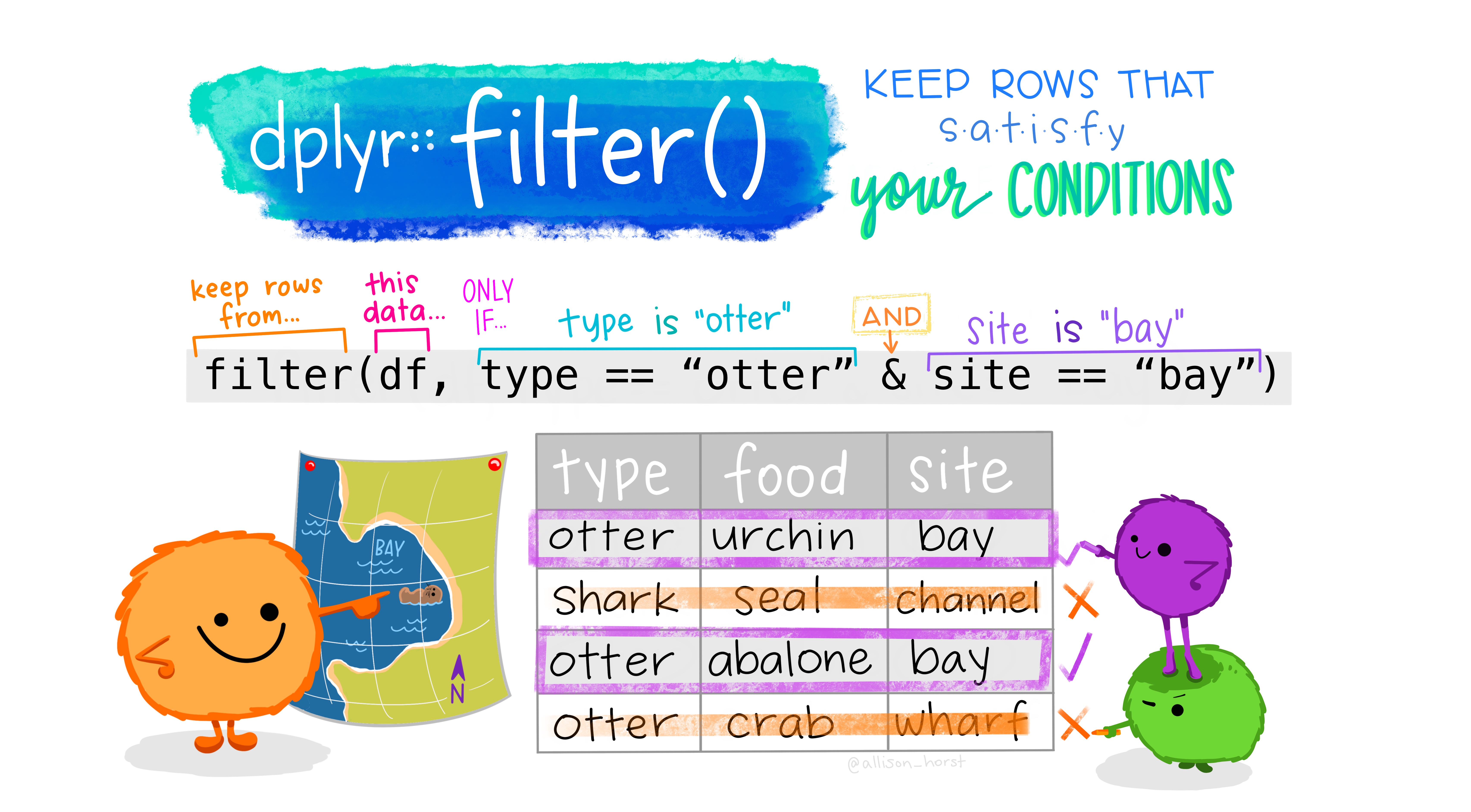
Filter out missing values before counting:
starwars %>%
  filter(!is.na(gender)) %>% # filter out missing values
  count(gender, sort = TRUE)
## # A tibble: 2 × 2
##   gender        n
##   <chr>     <int>
## 1 masculine    66
## 2 feminine     17
Count with respect to more than one variable:
starwars %>%
  count(species, gender, sort = TRUE) #
## # A tibble: 42 × 3
##    species  gender        n
##    <chr>    <chr>     <int>
##  1 Human    masculine    26
##  2 Human    feminine      9
##  3 Droid    masculine     5
##  4 <NA>     <NA>          4
##  5 Gungan   masculine     3
##  6 Mirialan feminine      2
##  7 Wookiee  masculine     2
##  8 Zabrak   masculine     2
##  9 Aleena   masculine     1
## 10 Besalisk masculine     1
## # … with 32 more rows
Weighted counting
You may want to use the wt argument to get a count weighted by another variable. Compare the call to count() with and without the wt argument in the example below. When wt = mass is used, we compute sum(mass) for each species, otherwise we compute the number of rows in each species:
starwars %>%
  count(species, wt = mass)
## # A tibble: 38 × 2
##    species       n
##    <chr>     <dbl>
##  1 Aleena       15
##  2 Besalisk    102
##  3 Cerean       82
##  4 Chagrian      0
##  5 Clawdite     55
##  6 Droid       279
##  7 Dug          40
##  8 Ewok         20
##  9 Geonosian    80
## 10 Gungan      148
## # … with 28 more rows
starwars %>%
  count(species)
## # A tibble: 38 × 2
##    species       n
##    <chr>     <int>
##  1 Aleena        1
##  2 Besalisk      1
##  3 Cerean        1
##  4 Chagrian      1
##  5 Clawdite      1
##  6 Droid         6
##  7 Dug           1
##  8 Ewok          1
##  9 Geonosian     1
## 10 Gungan        3
## # … with 28 more rows
You can add the counts to your tibble by using add_count(). Check out the n column:
starwars %>%
  add_count(species, wt = mass)
## # A tibble: 87 × 6
##    name               gender    species  mass height     n
##    <chr>              <chr>     <chr>   <dbl>  <int> <dbl>
##  1 Luke Skywalker     masculine Human      77    172 1821.
##  2 C-3PO              masculine Droid      75    167  279
##  3 R2-D2              masculine Droid      32     96  279
##  4 Darth Vader        masculine Human     136    202 1821.
##  5 Leia Organa        feminine  Human      49    150 1821.
##  6 Owen Lars          masculine Human     120    178 1821.
##  7 Beru Whitesun lars feminine  Human      75    165 1821.
##  8 R5-D4              masculine Droid      32     97  279
##  9 Biggs Darklighter  masculine Human      84    183 1821.
## 10 Obi-Wan Kenobi     masculine Human      77    182 1821.
## # … with 77 more rows
Complete counting
When you count with respect to two or more variables, it may happen that you don’t have all combinations. No worries, you’re covered with complete(). Compare the example below without and with the call to complete(). The Aleena species has no feminine representative, but this info is implicit. When complete() is used, a row is added with a NA for feminine gender:
starwars %>%
  filter(species %in% c('Aleena','Droid')) %>%
  count(species, gender)
## # A tibble: 3 × 3
##   species gender        n
##   <chr>   <chr>     <int>
## 1 Aleena  masculine     1
## 2 Droid   feminine      1
## 3 Droid   masculine     5
starwars %>%
  filter(species %in% c('Aleena','Droid')) %>%
  count(species, gender) %>%
  complete(species, gender)
## # A tibble: 4 × 3
##   species gender        n
##   <chr>   <chr>     <int>
## 1 Aleena  feminine     NA
## 2 Aleena  masculine     1
## 3 Droid   feminine      1
## 4 Droid   masculine     5
If you don’t like NA, you may use a 0 instead with the fill = list() argument:
starwars %>%
  filter(species %in% c('Aleena','Droid')) %>%
  count(species, gender) %>%
  complete(species, gender, fill = list(n = 0))
## # A tibble: 4 × 3
##   species gender        n
##   <chr>   <chr>     <dbl>
## 1 Aleena  feminine      0
## 2 Aleena  masculine     1
## 3 Droid   feminine      1
## 4 Droid   masculine     5
Computations across columns
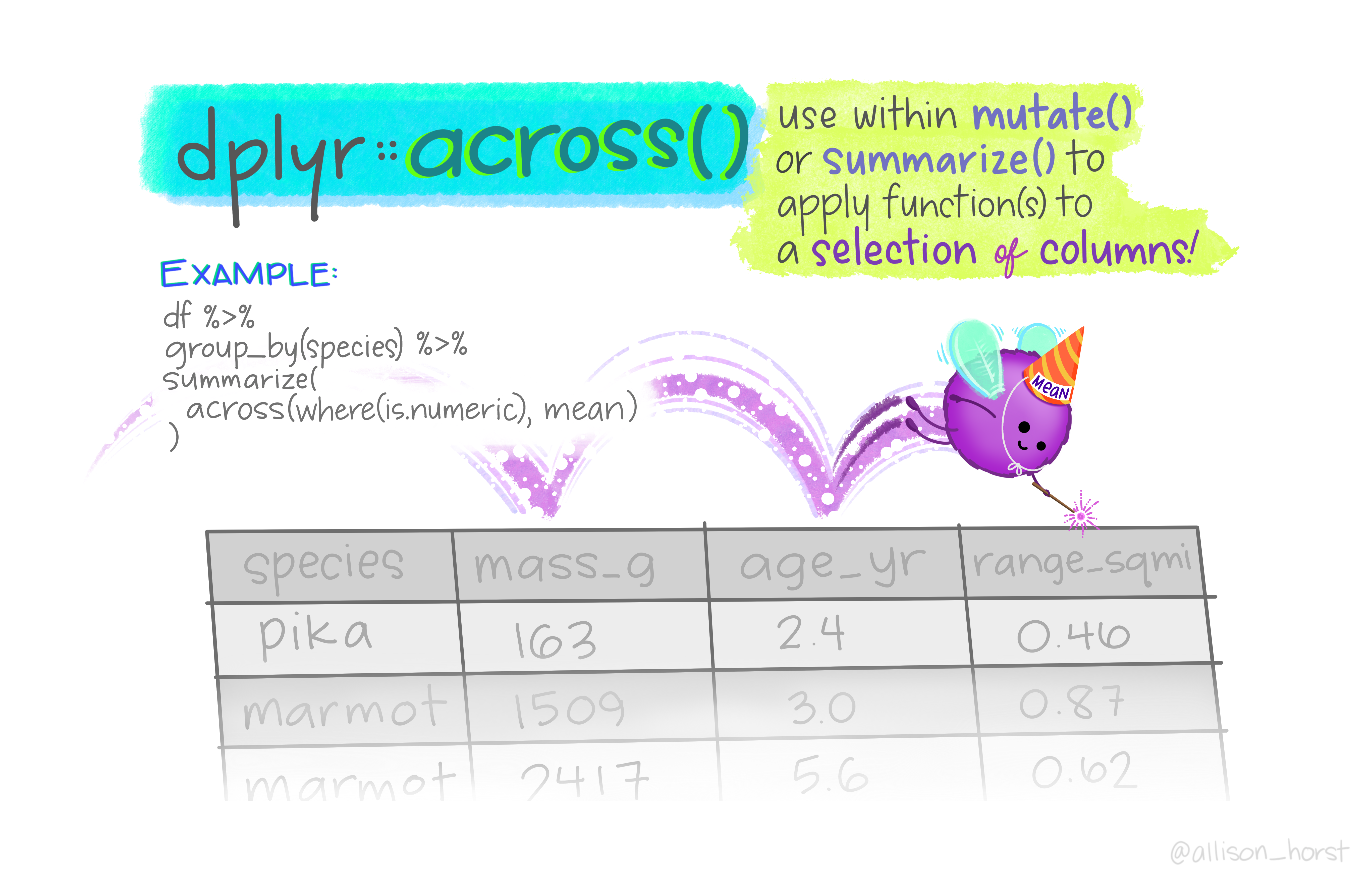
There is a function in dplyr which allows applying functions to columns of a dataset. In the example below, I compute the mean and standard deviation (storing them in a list) across all columns which have a numeric format (where(is.numeric)), while taking care of the missing values (na.rm = TRUE):
starwars %>%
  summarize(across(where(is.numeric),
                   list(mean = ~mean(.x, na.rm = TRUE),
                        sd = ~sd(.x, na.rm = TRUE))))
## # A tibble: 1 × 4
##   mass_mean mass_sd height_mean height_sd
##       <dbl>   <dbl>       <dbl>     <dbl>
## 1      97.3    169.        174.      34.8
Just use list(mean = mean, sd = sd) if you have no missing values. Also check out across(starts_with()) and across(everywhere()) for even more flexibility.
The decade trick
Probably the best of David Robinson’s tricks, he uses the integer division %/% to count things at coarse levels. For example, below is how you would count the number of characters in classes of height of width 10 centimeters.
starwars %>%
  count(height_classes = 10 * (height %/% 10))
## # A tibble: 18 × 2
##    height_classes     n
##             <dbl> <int>
##  1             60     1
##  2             70     1
##  3             80     1
##  4             90     4
##  5            110     1
##  6            120     1
##  7            130     1
##  8            150     3
##  9            160    10
## 10            170    15
## 11            180    20
## 12            190    12
## 13            200     4
## 14            210     2
## 15            220     3
## 16            230     1
## 17            260     1
## 18             NA     6
This trick also works for years count(year = 10 * (year %/% 10)), think of decades for example, hence the ‘decade trick’.
You may tune a bit the output by changing the name of the n column:
starwars %>%
  count(height_classes = 10 * (height %/% 10),
        name = "class_size")
## # A tibble: 18 × 2
##    height_classes class_size
##             <dbl>      <int>
##  1             60          1
##  2             70          1
##  3             80          1
##  4             90          4
##  5            110          1
##  6            120          1
##  7            130          1
##  8            150          3
##  9            160         10
## 10            170         15
## 11            180         20
## 12            190         12
## 13            200          4
## 14            210          2
## 15            220          3
## 16            230          1
## 17            260          1
## 18             NA          6
Lumping levels together
It has always been a nightmare to deal with factors in R. The package forcats is a game changer. For example, the function fct_lump() is useful to manipulate factors with many levels. You just lump levels together by preserving the n most common values, the other levels are lumped in a new Other level:
starwars %>%
  filter(!is.na(species)) %>%
  count(species = fct_lump(f = species, n = 3))
## # A tibble: 4 × 2
##   species     n
##   <fct>   <int>
## 1 Droid       6
## 2 Gungan      3
## 3 Human      35
## 4 Other      39
If you’d like to get rid of Other, just pipe a filter(species != 'Other').
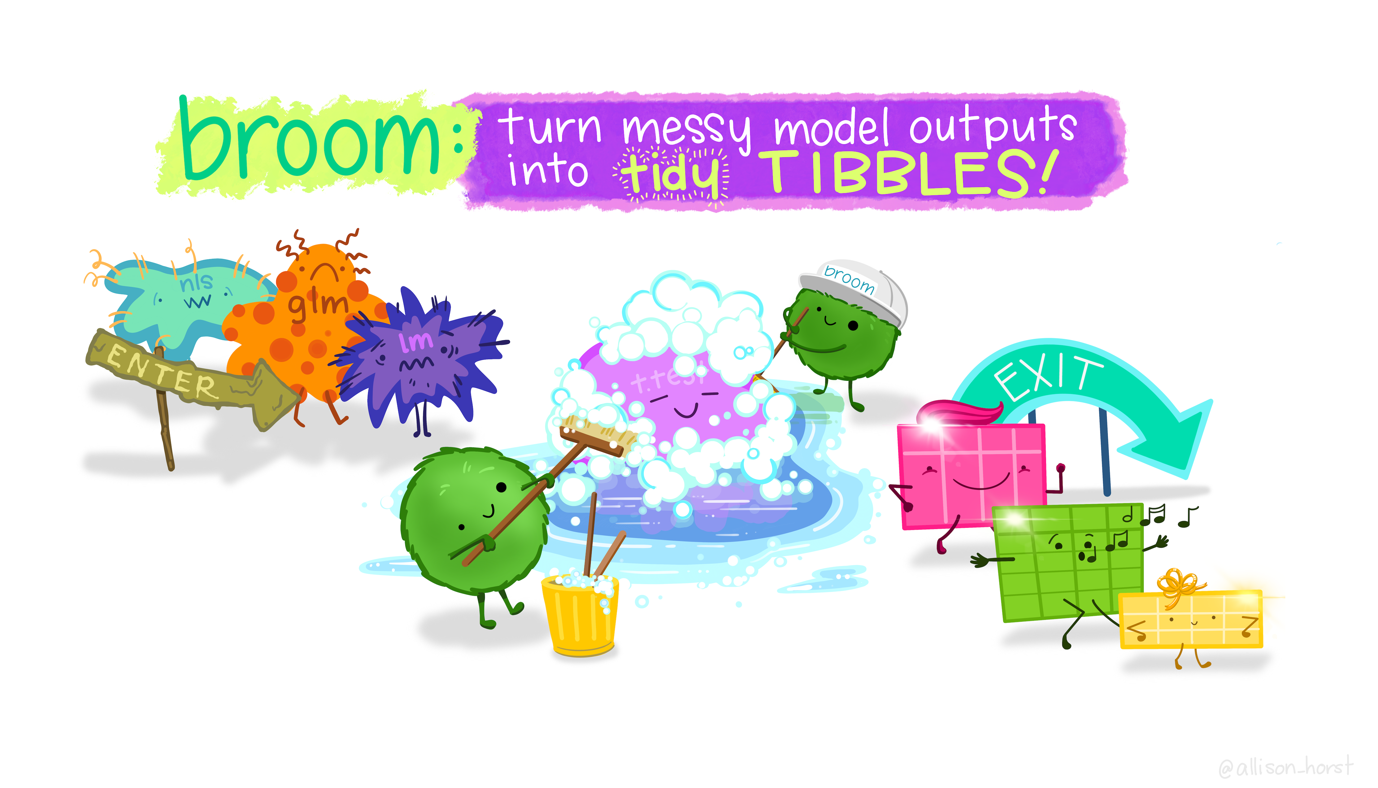
Pipe a (G)LM
Statistical analyses can easily be piped in your tidyverse workflow. You will find two simple examples below. Check out the broom package which cleans up the messy output of built-in R functions like lm() or glm().
Also, recommended is tidymodels a collection of packages for doing statistical analyses in the machine learning spirit. If you want to learn tidymodels by examples, I strongly recommend Julia Silge’s screencasts and her supervised machine learning course. The recent book Tidy Modeling with R is awesome, check it out!
Simple linear regression
starwars %>%
  lm(mass ~ height, data = .) %>%
  anova()
## Analysis of Variance Table
##
## Response: mass
##           Df  Sum Sq Mean Sq F value Pr(>F)
## height     1   29854   29854  1.0404  0.312
## Residuals 57 1635658   28696
Here is the tidy version of it:
starwars %>%
  lm(mass ~ height, data = .) %>%
  broom::tidy()
## # A tibble: 2 × 5
##   term        estimate std.error statistic p.value
##   <chr>          <dbl>     <dbl>     <dbl>   <dbl>
## 1 (Intercept)  -13.8     111.       -0.124   0.902
## 2 height         0.639     0.626     1.02    0.312
Get several summary statistics with function glance(), including the $R^2$ and the AIC:
starwars %>%
  lm(mass ~ height, data = .) %>%
  broom::glance()
## # A tibble: 1 × 12
##   r.squared adj.r.squared sigma statistic p.value    df logLik   AIC   BIC
##       <dbl>         <dbl> <dbl>     <dbl>   <dbl> <dbl>  <dbl> <dbl> <dbl>
## 1    0.0179      0.000696  169.      1.04   0.312     1  -386.  777.  783.
## # … with 3 more variables: deviance <dbl>, df.residual <int>, nobs <int>
Logistic regression
starwars %>%
  mutate(human = if_else(species == 'Human', 1, 0)) %>%
  glm(human ~ height, data = ., family = "binomial") %>%
  summary()
##
## Call:
## glm(formula = human ~ height, family = "binomial", data = .)
##
## Deviance Residuals:
##    Min      1Q  Median      3Q     Max
## -1.134  -1.025  -0.929   1.345   1.397
##
## Coefficients:
##              Estimate Std. Error z value Pr(>|z|)
## (Intercept) -1.025166   1.198297  -0.856    0.392
## height       0.003489   0.006715   0.520    0.603
##
## (Dispersion parameter for binomial family taken to be 1)
##
##     Null deviance: 104.83  on 77  degrees of freedom
## Residual deviance: 104.55  on 76  degrees of freedom
##   (9 observations effacées parce que manquantes)
## AIC: 108.55
##
## Number of Fisher Scoring iterations: 4
Here is the tidy version of it:
starwars %>%
  mutate(human = if_else(species == 'Human', 1, 0)) %>%
  glm(human ~ height, data = ., family = "binomial") %>%
  broom::tidy()
## # A tibble: 2 × 5
##   term        estimate std.error statistic p.value
##   <chr>          <dbl>     <dbl>     <dbl>   <dbl>
## 1 (Intercept) -1.03      1.20       -0.856   0.392
## 2 height       0.00349   0.00672     0.520   0.603
Let’s have a look to the fitted values and residuals with the function augment():
starwars %>%
  mutate(human = if_else(species == 'Human', 1, 0)) %>%
  glm(human ~ height, data = ., family = "binomial") %>%
  broom::augment()
## # A tibble: 78 × 9
##    .rownames human height .fitted .resid .std.resid   .hat .sigma .cooksd
##    <chr>     <dbl>  <int>   <dbl>  <dbl>      <dbl>  <dbl>  <dbl>   <dbl>
##  1 1             1    172  -0.425  1.36       1.37  0.0129   1.17 0.0102
##  2 2             0    167  -0.443 -0.996     -1.00  0.0135   1.17 0.00445
##  3 3             0     96  -0.690 -0.902     -0.937 0.0747   1.18 0.0219
##  4 4             1    202  -0.320  1.32       1.33  0.0211   1.17 0.0151
##  5 5             1    150  -0.502  1.40       1.41  0.0193   1.17 0.0166
##  6 6             1    178  -0.404  1.35       1.36  0.0130   1.17 0.00999
##  7 7             1    165  -0.450  1.37       1.38  0.0139   1.17 0.0112
##  8 8             0     97  -0.687 -0.903     -0.938 0.0732   1.18 0.0214
##  9 9             1    183  -0.387  1.35       1.35  0.0136   1.17 0.0103
## 10 10            1    182  -0.390  1.35       1.36  0.0135   1.17 0.0102
## # … with 68 more rows
Miscealleanous
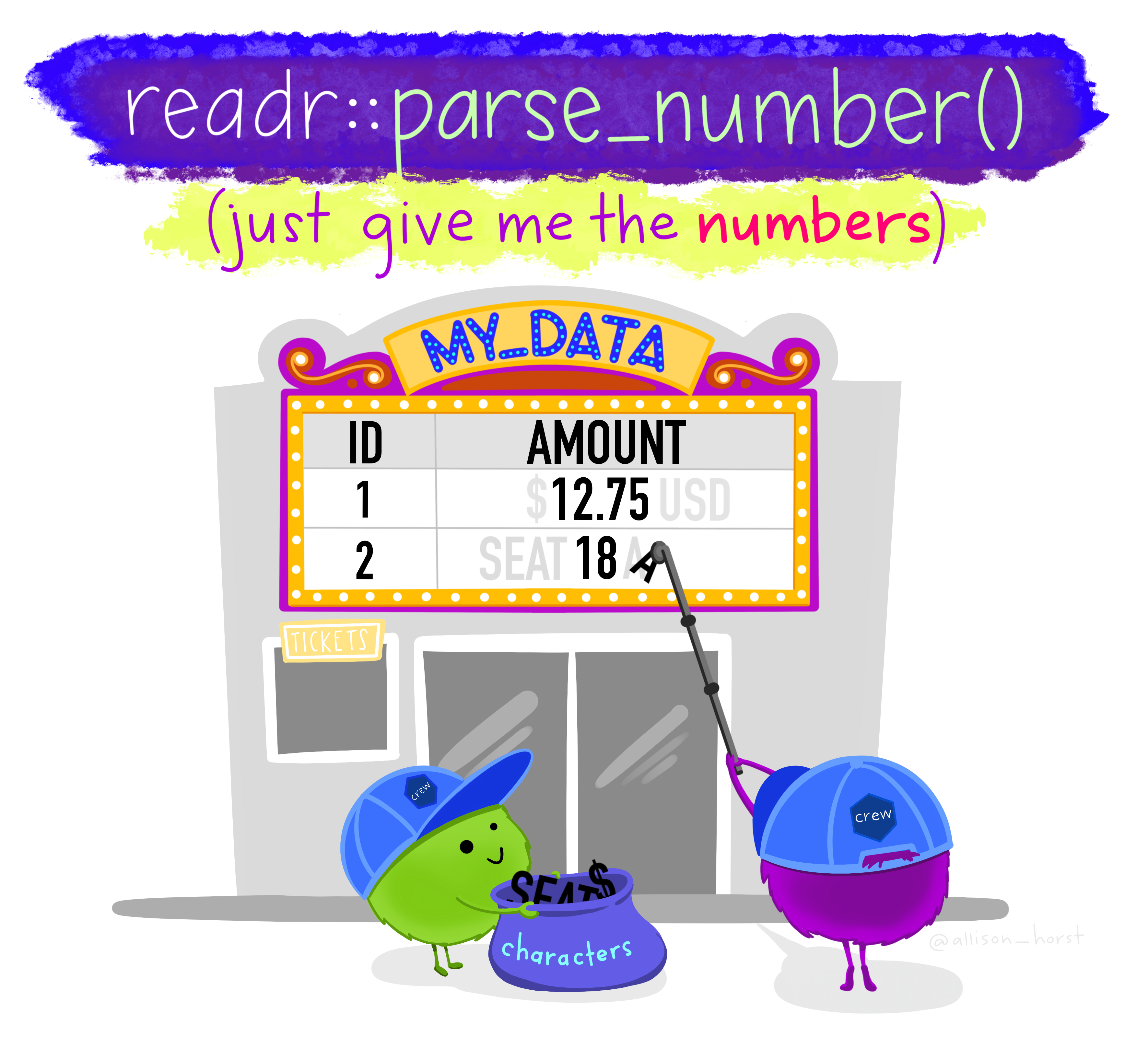
?parse_number
parse_number("$1000")
## [1] 1000
parse_number("1,234,567.78")
## [1] 1234568
Data visualisation
Ordering bars in a bar plot
Compare:
starwars %>%
  filter(!is.na(species)) %>%
  count(species = fct_lump(species, 3)) %>%
  ggplot(aes(x = n, y = species)) +
  geom_col()

with:
starwars %>%
  filter(!is.na(species)) %>%
  count(species = fct_lump(species, 3)) %>%
  mutate(species = fct_reorder(species, n)) %>%
  ggplot(aes(x = n, y = species)) +
  geom_col()

We have reordered the species factor by n which is created by the call to count(), and the Droid and Gungan species get ordered adequately. Neat isn’t it?! The function fct_reorder() is another nice feature of the forcats package.
Ordering bars within bar plots
When we use facet_wrap() to get a barplot for each level of a factor, the reordering should apply within the levels of this factor. The fct_reorder() call above won’t work:
starwars %>%
  filter(!is.na(species)) %>%
  count(species = fct_lump(species, 5),
        gender) %>%
  mutate(species = fct_reorder(species, n)) %>%
  ggplot(aes(x = n, y = species)) +
  geom_col() +
  facet_wrap(vars(gender))

There is exactly what we need in the tidtext package. This is the function reorder_within() which works with scale_y_reordered:
library(tidytext)
starwars %>%
  filter(!is.na(species)) %>%
  count(species = fct_lump(species, 5),
        gender) %>%
  mutate(species = reorder_within(species, n, gender)) %>%
  ggplot(aes(x = n, y = species)) +
  geom_col() +
  scale_y_reordered() +
  facet_wrap(vars(gender))

Little tricks I always forget about
Free the scales
The argument scales = "free" is useful when using facet_wrap(). It allows the X and Y axes to have their own scale in each panel. You can choose to have a free scale on the X axis only with scales = "free_x", same thing for the Y axis with scales = "free_y".
Flip coordinates
We used to add a coord_flip() following geom_col() to improve the reading of a bar plot by having the categories on the Y axis. This extra line of code is no longer needed as we can simply permute the variables in the aes().
Titles too long
Also, in a facet_wrap(), the title of each panel might be too long so that it doesn’t read properly. There are two ways to fix that. Either you decrease the font size with a theme(strip.text = element_text(size = 6)) or you truncate the title with a mutate(tr_title_text = str_trunc(title_text, 25).
Log scale
It often makes sense to plot your data using log scales. It is very easy to do in ggplot2 by piping a scale_x_log10() or a scale_y_log10().
Axes format
To improve the reading of your figure, it might be useful to represent the unit of an axis in percentage or display numbers with commas. The scales package is what you need. For example, pipe a scale_y_continuous(labels = scales::percent) to have your Y axis in percentages, or
scale_x_continuous(labels = scales::comma) to add commas to the numbers of your X axis.
Legend of a map
To draw maps, Dave Robinson uses the sf package. Check out the official site. In case you’re interested in, I wrote an introduction to GIS and mapping in R using the sf package.
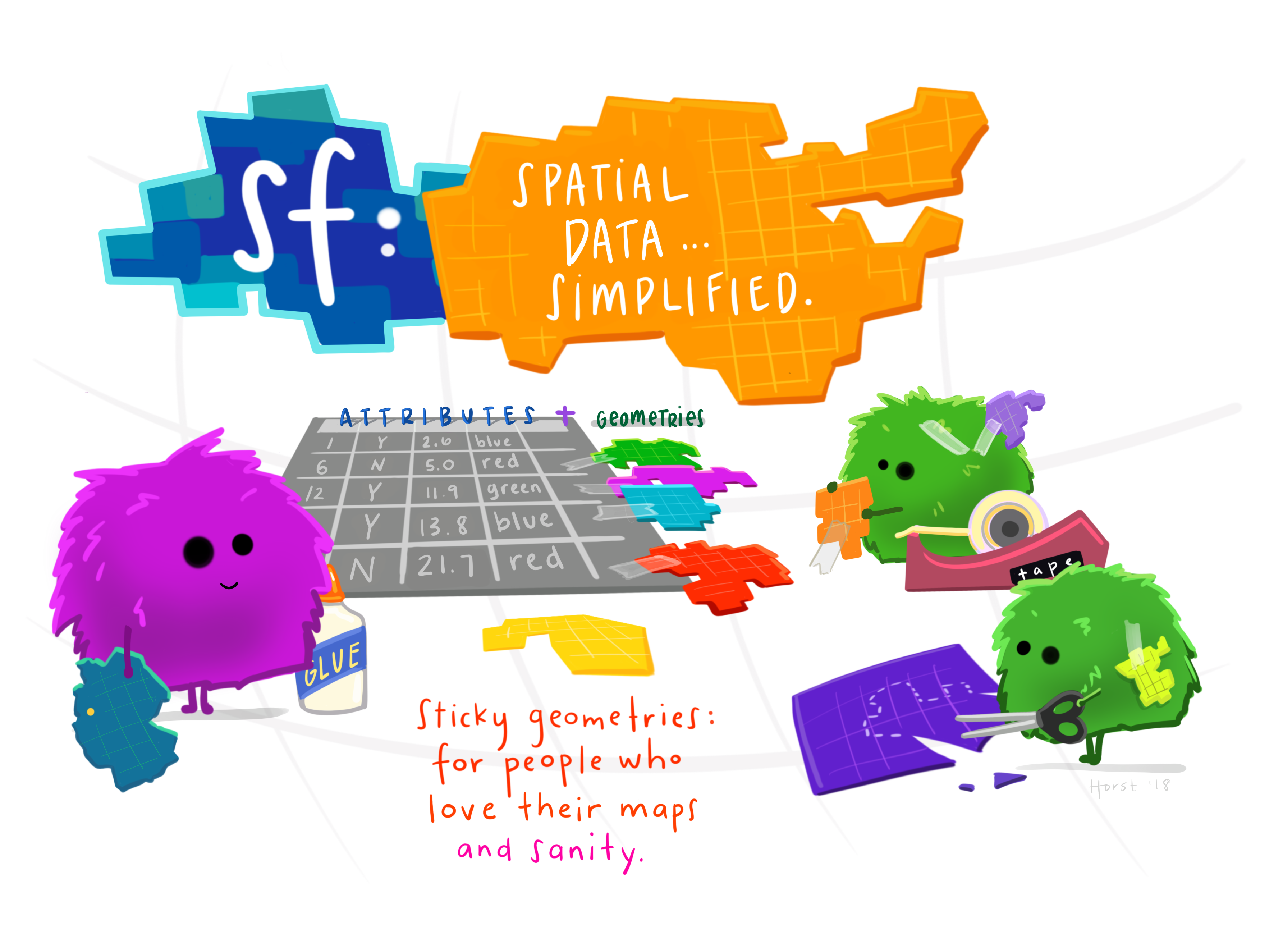
When I use maps, I always forget how to tune the legend. The scale_fill_gradient2() function is great in that it allows defining colors for low and high ends of the gradient (e.g. low = "brown", high = "darkgreen"), and the midpoint of the diverging scale (e.g. midpoint = .1).
Stuff I need to learn
David Robinson uses a bunch of tools that he has perfectly internalised so that he doesn’t have to go back and forth between RStudio and the internet to find how to wrangle this or plot that. I am faaaaaaaaaaar from having his level of expertise. I have identified a few things I need to learn to improve myself.
Regular expressions
I find them boring but regular expressions for describing patterns in strings are very useful when you have to filter rows based on some patterns (str_detect()), remove characters (str_remove()) or separate rows (separate_rows()). Good resources are this book chapter dedicated to strings and the vignette of the stringr package.
Web scraping
When you analyse data, sometimes you need some extra information that can be extracted from the internet. The rvest package helps you scrape information from web pages. The official site is a good starting point.
Animation
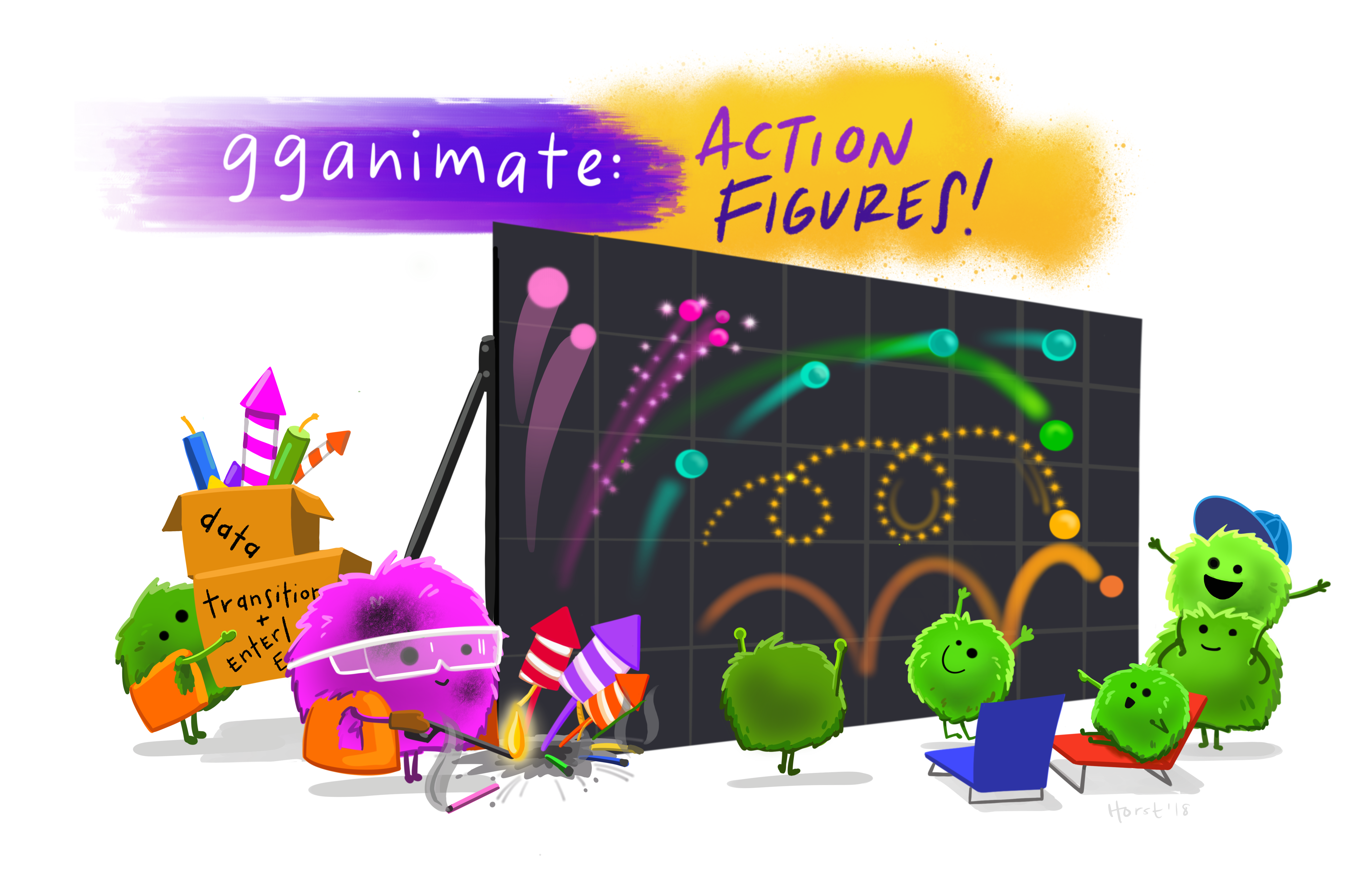
It is relatively easy to animate a plot (whatever you have made: boxplots, scatter plots, maps, etc) using the gganimate package. Check out the official site.
Networks
Another great package by Thomas Lin Pedersen is ggraph to visualise data that are structured in relations like networks and trees. Check out the official site.
Dimensional modeling
The cross by functions look terrific to aggregate data by calendar dates. I need to understand how to work with them. Check out the official site and this talk by Kaelen Medeiros.