Reconstruction de trajectoires et identification de comportements à partir de données de géolocalisation
M.-P. Etienne, P. GLoaguen
Packages à charger
rm(list = ls())
library(tidyverse) # Pour la manipulation de données
library(ggpubr)
library(ggmap)
library(sf) # Pour les objets spatiaux
library("rnaturalearth") # Pour les cartes
library(lubridate) # Pour les dates
library(nlme) # Pour l'estimation
source(file = 'code/utils_HMM.R')
source(file = 'code/utils_ICL.R')
library(moveHMM)
library(depmixS4)
library(circular)
library(MARSS)
Les données
On lit les données.
fou_dta <- read.table("dat/donnees_fous.txt", sep = ";", header = TRUE)Carte du monde.
world <- ne_countries(scale = "medium", returnclass = "sf") %>%
  st_crop(c(xmin = -90, ymin = -60, xmax = -30, ymax = 15))

zone_contour <-  fou_dta %>%
  st_as_sf(coords = c("lon", "lat") ) %>%
  st_set_crs(4326) %>%
  st_bbox() %>%
  # {. * c(0.99, 0.99, 1.01, 1.01)} %>%
  st_as_sfc()

world_plot <- world  %>%
  ggplot() +
  geom_sf(fill = "#c9d0a3") +
  geom_sf(data = zone_contour, fill = "white", color = "red") +
  theme(panel.background = element_rect(fill = "#99b3cc"))
La trajectoire.
zone_box <- c(-32.75, -4.7, -31.8, -3.75)
zone_map <- ggmap::get_stamenmap(bbox = zone_box,
                                 zoom = 10)
traj_plot <- ggmap::ggmap(zone_map) +
    labs(x = "Longitude", y = "Latitude") +
    geom_path(data = fou_dta, aes(x = lon, y = lat, color = ID)) +
  theme(legend.position = "none", axis.text = element_blank(),
        axis.ticks = element_blank(),
        axis.title = element_blank())
On visualise.
gridExtra::grid.arrange(world_plot, traj_plot, nrow = 1)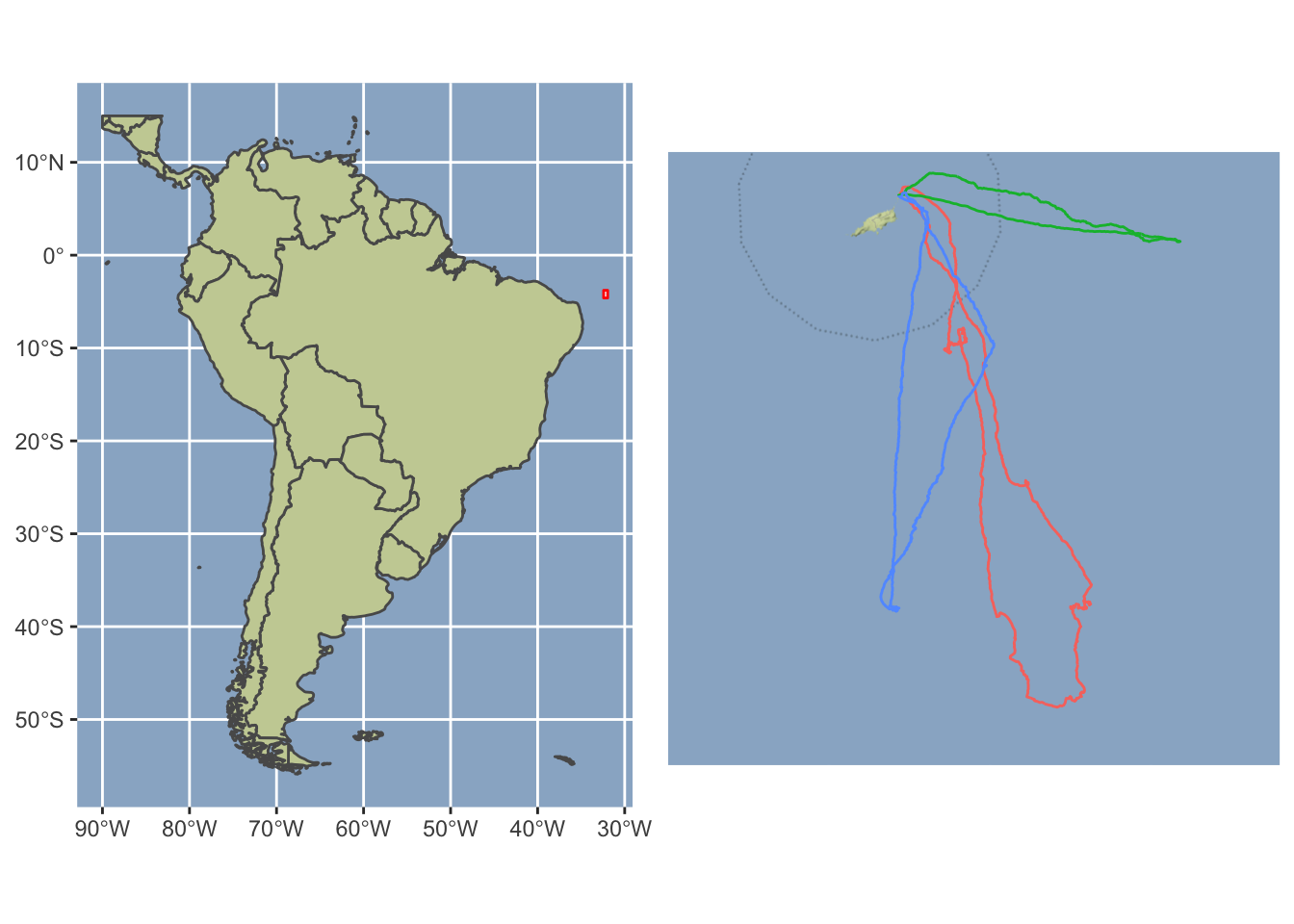
Projection.
fou_dta_utm <- fou_dta %>%
  st_as_sf(coords = c("lon", "lat")) %>%
  mutate(dist_scaled = scale(dist.nid),
         dist_scaled_sq = dist_scaled^2,
         all_scaled = scale(alt)) %>%
  st_set_crs(4326)  %>%
  st_transform(crs=32725) %>%
  mutate(Easting = st_coordinates(.)[,"X"],
         Northing = st_coordinates(.)[,"Y"])
Kalman smoothing
On lisse par individu
smoothing_function <- function(utm_data_){
  MARSS_data <- utm_data_ %>%
    as.data.frame() %>% # leaving sf format
    dplyr::select(x = Easting, y = Northing) %>%
    as.matrix() %>%
    t()
  model_list <- list(B = diag(1, 2), Z = diag(1, 2),
                     x0 = MARSS_data[,1, drop = FALSE],
                     V0 = diag(1, 2),
                     U = matrix(0, nrow = 2),
                     A = matrix(0, nrow = 2),
                     Q = matrix(list("q1", 0, 0, "q2"), 2, 2),
                     C = matrix(0, 2, 2),
                     c = matrix(0, 2, 1),
                     G = diag(1, 2),
                     D = diag(0, 2),
                     d = matrix(0, 2, 1),
                     # R = matrix(list("r", 0, 0, "r"), 2, 2),
                     R = diag(3, 2)) # Erreur standard de 1 metres
  MLEobj <- MARSS(MARSS_data, model = model_list,
                  control = list(maxit = 1e3))

  # MARSSkf needs a marss MLE object with the par element set
  MLEobj$par <- MLEobj$start
  # Compute the kf output at the params used for the inits
  kfList <- MARSSkfss(MLEobj)
  output <- utm_data_ %>%
    mutate(Easting_smoothed = kfList$xtT[1, ],
           Northing_smoothed = kfList$xtT[2, ])  %>%
    as_tibble() %>%
    dplyr::select(-geometry)
  return(output)
}
Lissage Kalman
fou_dta_utm_smoothed <- map_dfr(split(fou_dta_utm,
                                      fou_dta_utm$ID),
                                smoothing_function)
## Success! abstol and log-log tests passed at 16 iterations.
## Alert: conv.test.slope.tol is 0.5.
## Test with smaller values (<0.1) to ensure convergence.
##
## MARSS fit is
## Estimation method: kem
## Convergence test: conv.test.slope.tol = 0.5, abstol = 0.001
## Estimation converged in 16 iterations.
## Log-likelihood: -36300.97
## AIC: 72605.94 AICc: 72605.94
##
## Estimate
## Q.q1 2747
## Q.q2 7837
## Initial states (x0) defined at t=0
##
## Standard errors have not been calculated.
## Use MARSSparamCIs to compute CIs and bias estimates.
##
## Success! abstol and log-log tests passed at 16 iterations.
## Alert: conv.test.slope.tol is 0.5.
## Test with smaller values (<0.1) to ensure convergence.
##
## MARSS fit is
## Estimation method: kem
## Convergence test: conv.test.slope.tol = 0.5, abstol = 0.001
## Estimation converged in 16 iterations.
## Log-likelihood: -9378.381
## AIC: 18760.76 AICc: 18760.77
##
## Estimate
## Q.q1 18678
## Q.q2 2557
## Initial states (x0) defined at t=0
##
## Standard errors have not been calculated.
## Use MARSSparamCIs to compute CIs and bias estimates.
##
## Success! abstol and log-log tests passed at 16 iterations.
## Alert: conv.test.slope.tol is 0.5.
## Test with smaller values (<0.1) to ensure convergence.
##
## MARSS fit is
## Estimation method: kem
## Convergence test: conv.test.slope.tol = 0.5, abstol = 0.001
## Estimation converged in 16 iterations.
## Log-likelihood: -21117.56
## AIC: 42239.11 AICc: 42239.11
##
## Estimate
## Q.q1 2685
## Q.q2 9278
## Initial states (x0) defined at t=0
##
## Standard errors have not been calculated.
## Use MARSSparamCIs to compute CIs and bias estimates.Plot smoothing.
fou_dta_utm_smoothed %>%
  dplyr::select(Easting, Easting_smoothed, Northing, Northing_smoothed) %>%
  unite(col = "Raw", Easting, Northing, sep = "-") %>%
  unite(col = "Smoothed", Easting_smoothed, Northing_smoothed, sep = "-") %>%
  gather(key = "Trajectoire", value = "Coordonnees",
         factor_key = TRUE) %>%
  separate(col = Coordonnees, into = c("Longitude", "Latitude"),
           sep = "-", convert = TRUE) %>%
  mutate(Trajectoire = factor(Trajectoire, labels = c("Brute", "Lissée"))) %>%
  ggplot() +
  aes(x = Longitude, y = Latitude, color = Trajectoire) +
  geom_path() +
  coord_cartesian(ylim = c(955, 956) * 1e4, xlim = c(575, 580) * 1e3) +
  theme(axis.text = element_blank(), axis.ticks = element_blank(),
        axis.title = element_blank())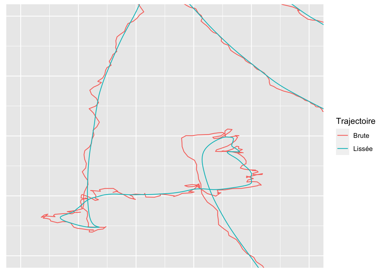
Utilisation du package moveHMM.
Metric Step Length/ Turning angle is implemented is the moveHMM package.
moveHMM_data <- fou_dta_utm_smoothed %>%
  as.data.frame() %>%
  rowid_to_column( var = "id_point") %>%
  dplyr::select(ID, id_point, time_step, Easting, Northing,
                Easting_smoothed, Northing_smoothed,
                alt_scaled, dist_scaled, dist_scaled_sq) %>%
 moveHMM::prepData(type = "UTM", coordNames = c("Easting_smoothed",
                                                "Northing_smoothed"))
Utilisation du package depmix.
Gaussian emission HMM is implemented in the depmixS4 package.
Creation de v_p/v_r
depmix_data <- moveHMM_data %>%
  as_tibble() %>%
  mutate(v_p = step * cos(angle), v_r = step * sin(angle)) %>%
  replace_na(list(angle = 0, v_r = 0)) %>%
  mutate(v_p = ifelse(is.na(v_p), step, v_p))
# Distinguishing animals
n_times <- depmix_data %>%
  group_by(ID) %>%
  summarise(n_times = n()) %>%
  pull(n_times)
Modèle initial.
n_states <- 3
set.seed(123)
initial_model <- depmixS4::depmix(list(v_p ~ 1, v_r ~ 1), data = depmix_data,
                                                nstates = n_states,
                         family = list(gaussian(), gaussian()), ntimes = n_times,
                         respstart = get_init_depmix(depmix_data, nbStates = n_states),
                         initdata = rep(1/n_states,n_states),
                         transition = ~ 1)
depmix_fit <- depmixS4::fit(initial_model,
                            verbose = FALSE,
                            emcontrol = em.control(crit = "relative"))
## converged at iteration 78 with logLik: -35517.53Résultats.
States labelling is arranged according the the mean step length.
rank_vector_depmix <-  posterior(depmix_fit) %>%
  dplyr::select(state) %>%
  mutate(step = depmix_data$step) %>%
  group_by(state) %>%
  summarise(mean_step = mean(step, na.rm = T)) %>%
  arrange(state) %>%
  pull(mean_step) %>%
  rank()
depmix_states <- posterior(depmix_fit) %>%
  rename(Predicted_state = state) %>% # So that it do not start with s
  rename_at(.vars = vars(starts_with("S")),
            function(name) paste0("State",rank_vector_depmix[str_extract(name, "[[::0-9::]]") %>%
                                                               as.numeric()])) %>%
  mutate(Predicted_state = rank_vector_depmix[Predicted_state]  %>%
           factor(levels = 1:n_states)) %>%
  bind_cols(depmix_data, .) %>%
  # rename(Easting = x, Northing = y) %>%
  as_tibble() %>%
  mutate(metric = "Vitesse bivariée")
moveHMM_fit
par_init_moveHMM <- get_init_moveHMM(dta = moveHMM_data, nbStates = n_states)
set.seed(123)
moveHMM_fit <- moveHMM::fitHMM(data = moveHMM_data, nbStates = n_states,
                              stepPar0 = par_init_moveHMM$stepPar0,
                              anglePar0 = par_init_moveHMM$anglePar0,
                              formula = ~ 1)
moveHMM_results
rank_vector_moveHMM <-  tibble(state = moveHMM::viterbi(moveHMM_fit)) %>%
  mutate(step = depmix_data$step) %>%
  group_by(state) %>%
  summarise(mean_step = mean(step, na.rm = T)) %>%
  arrange(state) %>%
  pull(mean_step) %>%
  rank()
moveHMM_states <- moveHMM::stateProbs(moveHMM_fit) %>%
  as_tibble() %>%
  rename_at(.vars = vars(starts_with("V")),
            function(name) paste0("State",rank_vector_moveHMM[str_extract(name, "[[::0-9::]]") %>%
                                                               as.numeric()])) %>%
  bind_cols(depmix_data, .) %>%
  mutate(Predicted_state = rank_vector_moveHMM[moveHMM::viterbi(moveHMM_fit)] %>%
           factor(levels = 1:n_states)) %>%
  mutate(metric = "Longueur/Angle")
ICL(moveHMM_fit)
##
## Hidden contribution : -299.0032
## Emission contribution : -11762.89## [1] 24210.59Etats estimés.
estimated_states <- moveHMM_states %>%
  bind_rows(depmix_states)
Visualise états prédits.
estimated_states %>%
  group_by(ID, metric) %>%
  mutate(Next_East = lead(x), Next_North = lead(y)) %>%
  ggplot(aes(x = x, y = y)) +
  # geom_point(aes(y = Value, color = Predicted_state)) +
  geom_segment(aes(xend = Next_East, yend = Next_North,
                   color = Predicted_state,
                   group = interaction(metric, ID, linetype = ID))) +
  # geom_point(aes(y = Value, color = Predicted_state)) +
  facet_wrap( ~ metric) +
  labs(color = "Etat prédit") +
  theme(axis.title = element_blank(), axis.text = element_blank(),
        axis.ticks = element_blank())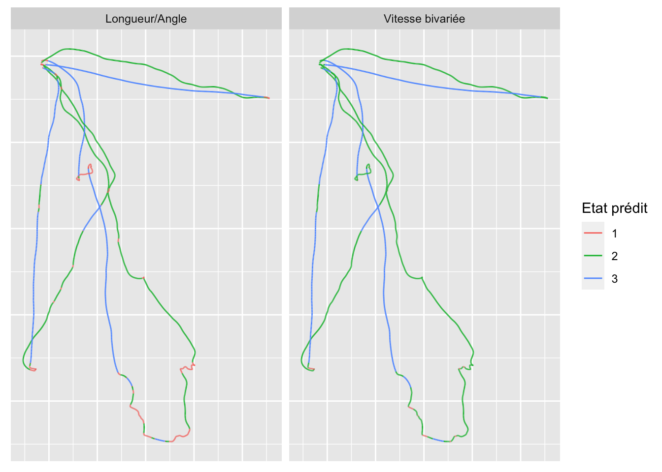
Plot distribution steps
plot_distrib_steps <- estimated_states %>%
  ggplot(aes(x = step)) +
  geom_density(aes(fill = Predicted_state), alpha = 0.5) +
  facet_wrap(~metric) +
  labs(y = "Densité estimée", x = "", title = "Longueurs de pas",
       fill = "Etat prédit")
Plot distribution angles
plot_distrib_angles <-  estimated_states %>%
  ggplot(aes(x = angle * 180 / pi)) +
    coord_polar(theta = "x", start = pi/2 , direction = -1, clip = "off") +
  facet_wrap(~ metric) +
  geom_histogram(aes(fill = Predicted_state, y = ..density..),
                 breaks = seq(-180, 180, by = 15), color = "black",
                  alpha = 0.5,
                  position = "identity") +
  scale_x_continuous(breaks = seq(-180, 180, by = 15), expand = c(0, 0)) +
  theme(axis.ticks = element_blank(), axis.title = element_blank(),
        axis.text.y = element_blank()) +
  labs(fill = "Etat prédit", title = "Angles")
Plot distributions
gridExtra::grid.arrange(plot_distrib_steps, plot_distrib_angles, nrow = 2)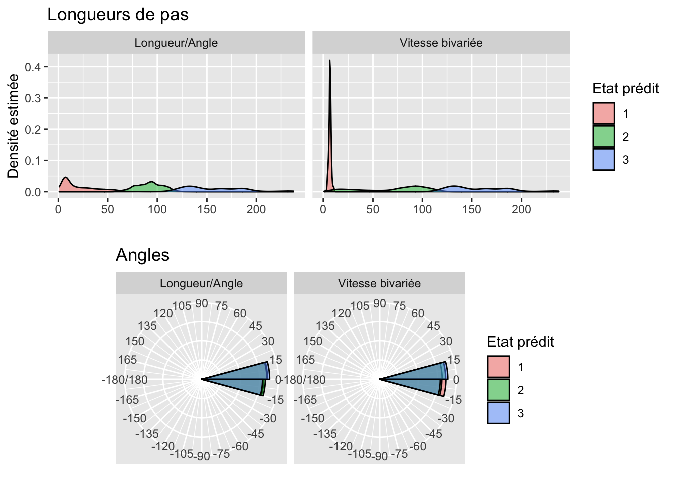
contingence etats
get_contingency <- function(ID_){
  state_sl <- filter(moveHMM_states, ID %in% ID_) %>%
    pull(Predicted_state)
  state_bv <- filter(depmix_states, ID %in% ID_) %>%
    pull(Predicted_state)
  contingency_table <- table(state_sl, state_bv) %>%
    prop.table(margin = 2) %>%
    as_tibble() %>%
    # mutate(ID = ID_) %>%
    rename(Freq = n)
}
contingency_tibble <- estimated_states %>%
    pull(ID) %>%
    unique() %>%
    get_contingency()
contingency_tibble %>%
    mutate(state_bv = factor(state_bv, levels = paste(3:1))) %>%
    ggplot(aes(state_sl, state_bv)) +
    geom_tile(aes(fill = Freq)) +
    # facet_wrap(~ID) +
    geom_text(aes(label = round(Freq, 2)), color = "red") +
    scale_fill_viridis_c(name = "Proportion") +
    labs(x = "Longueur/Angle", y = "Vitesse bivariée", title = "Contingence des états") +
    scale_x_discrete(expand = c(0, 0)) +
    scale_y_discrete(expand = c(0, 0))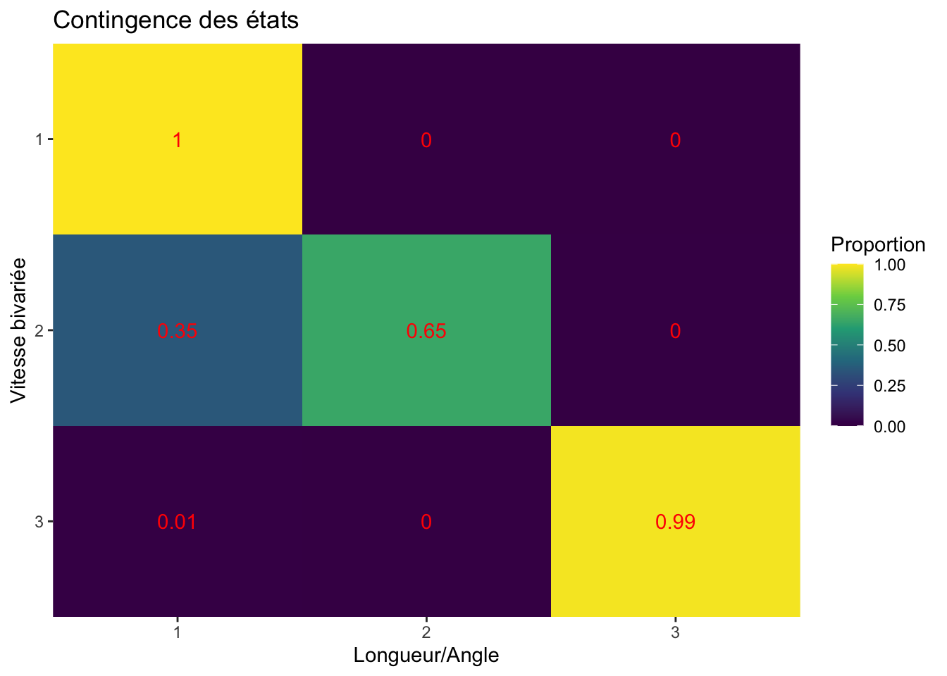
Probabilite etat aposteriori
estimated_states %>%
  filter(ID == "BR1705") %>%
  dplyr::select(time_step, metric, State1, State2) %>%
  gather(-time_step, -metric, key = "Etat", value = "Proba") %>%
  mutate(Etat = str_extract(Etat, "[[::0-9::]]")) %>%
  ggplot(aes(x = time_step, y = Proba)) +
  geom_line(aes(color = Etat), alpha = 0.5, size = 1.2) +
  labs(color = "Etat", y = "Probabilité", x = "Pas de temps") +
  facet_wrap(~metric)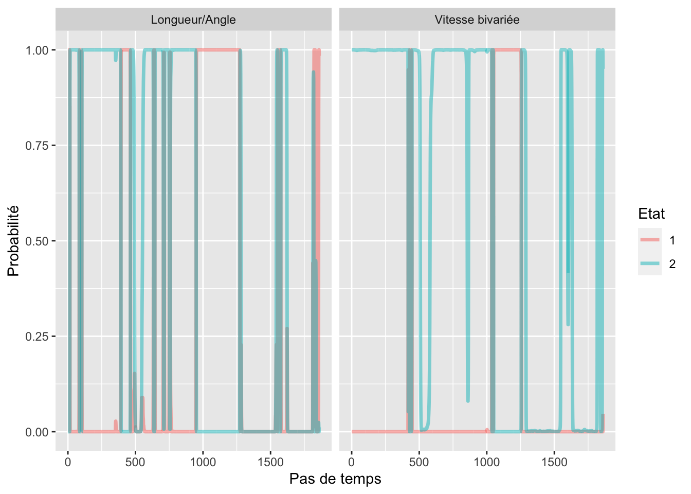
Modèle avec covariable
Définition des paramètres initiaux (fastidieux)
mat_from_1 <- c(10, 0.5, 0.5,
                0, 1, 1
                ,0, 1, 1
)
mat_from_2 <- c(10, 0.5, 0.001,
                0, 1, 0.001
                ,0, 1, 0.001
)
mat_from_3 <- c(10, 0.001, 0.5,
                0, 0.001, 1
                ,0, 0.001, 1
)
trans_inits <-  c(mat_from_1, mat_from_2, mat_from_3)
fixed_parameters <- c(rep(TRUE, 3), # Distribution initiale
                      trans_inits %in% c(0, 10),
                      rep(FALSE, 12))
initial_model_covariates <- depmixS4::depmix(list(v_p ~ 1, v_r ~ 1),
                                             data = depmix_data,
                                             nstates = 3,
                                             family = list(gaussian(), gaussian()),
                                             ntimes = n_times,
                                             respstart = getpars(depmix_fit)[13:24],
                                             trstart = trans_inits,
                                             instart = rep(1/3, 3),
                                             transition = ~ dist_scaled + dist_scaled_sq)

depmix_fit_covariates <- depmixS4::fit(initial_model_covariates, verbose = FALSE,
                                       fixed = fixed_parameters,
                                       emcontrol = em.control(crit = "absolute"))
##
## Iter: 1 fn: 35509.6490 Pars: -28.029922 -6.022884 7.379797 0.350806 -22.937094 1.179394 27.857595 24.039215 27.967898 26.892274 36.864200 37.342470 -0.081545 5.910703 0.441220 -0.212335 0.213694 0.037421 156.081821 29.703281 0.250873 1.560060 6.768905 1.202913 -0.008824 0.125724 70.589818 32.787378 -0.009771 1.726769
## Iter: 2 fn: 35509.6490 Pars: -28.030240 -6.022809 7.379897 0.350924 -22.937428 1.179325 27.857710 24.038955 27.968389 26.893164 36.864716 37.342589 -0.082490 5.909983 0.440826 -0.212461 0.214089 0.037761 156.083129 29.702884 0.250871 1.560038 6.768896 1.202927 -0.008824 0.125724 70.590161 32.787477 -0.009770 1.726771
## solnp--> Completed in 2 iterationsbetas <- purrr::map(depmix_fit_covariates@transition,
function(x) x@parameters$coefficients)
get_probs <- function(beta_){
x_ <- seq(-1.75, 1.75, length.out = 1001)
my_X <- tibble(Int = rep(1, 1001),
x = x_,
x2 = x^2) %>%
as.matrix()
x_beta <- my_X %*% beta_
Pr1 <- apply(x_beta, 1, function(x) 1 / (1 + sum(exp(x[2:3]))))
Pr23 <- exp(x_beta[, 2:3]) * Pr1
cbind(Pr1, Pr23) %>%
as.data.frame() %>%
mutate(d = x_) %>%
tidyr::pivot_longer(cols = -d,
names_to = "to",
values_to = "Prob") %>%
mutate(to = factor(to,
levels = c("Pr1", "St2", "St3"),
labels = paste0(1:3)))
}
map_dfr(betas, get_probs, .id = "from") %>%
ggplot(aes(x = d, y = Prob)) +
facet_grid(from ~ to, switch = "y") +
geom_line() +
labs(x = "Distance au nid", y = "Probabilité de transition")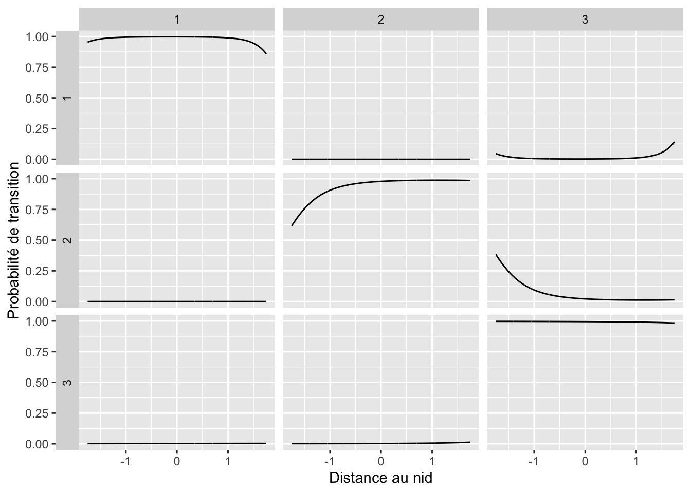
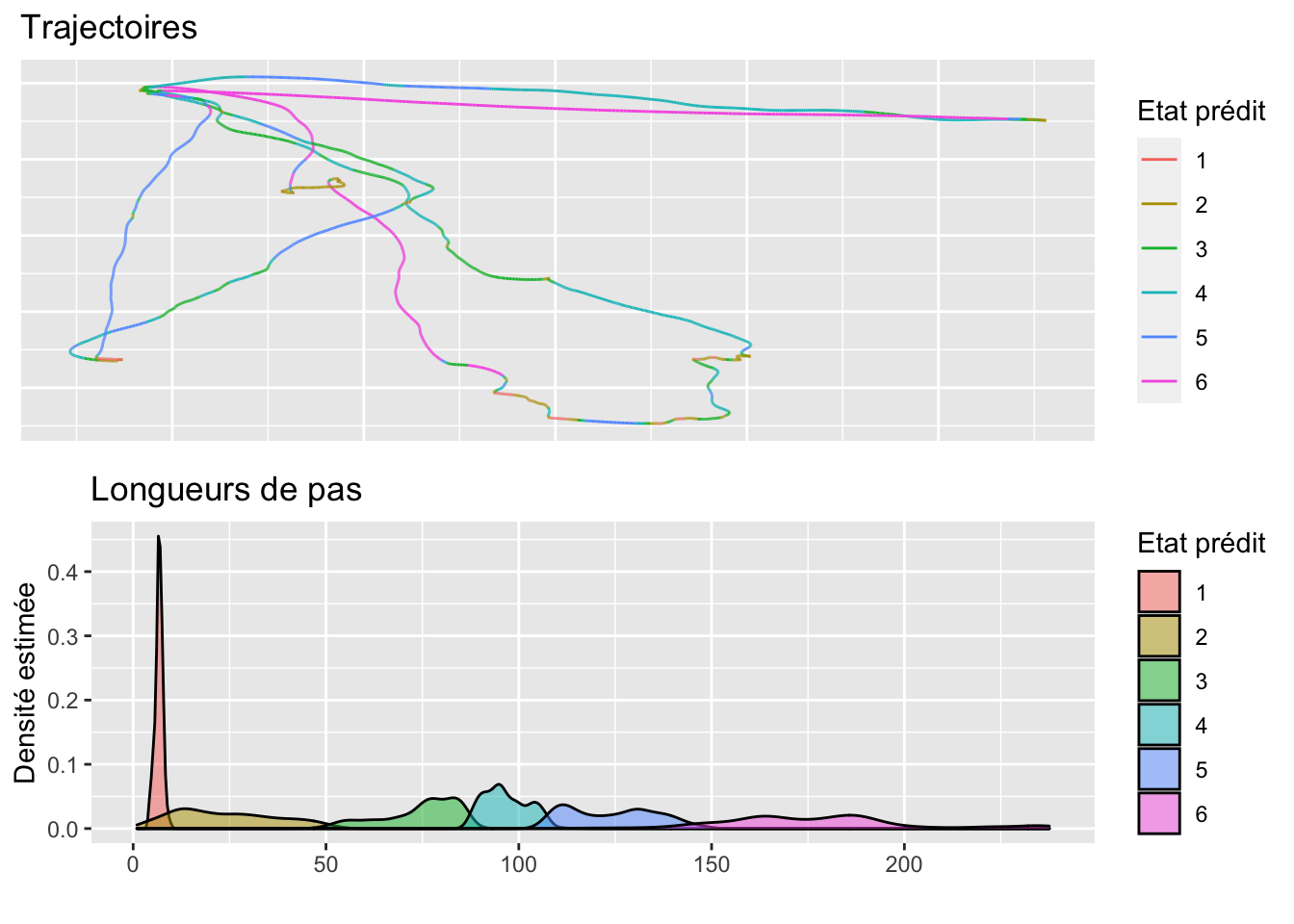
Modèle à 6 états
n_states <- 6
set.seed(123)
initial_model_J6 <- depmixS4::depmix(list(v_p ~ 1, v_r ~ 1), data = depmix_data,
                                                nstates = n_states,
                         family = list(gaussian(), gaussian()), ntimes = n_times,
                         respstart = get_init_depmix(depmix_data, nbStates = n_states),
                         initdata = rep(1/n_states,n_states),
                         transition = ~ 1)
depmix_fit_J6 <- depmixS4::fit(initial_model_J6,
                            verbose = FALSE,
                            emcontrol = em.control(crit = "relative"))
## converged at iteration 37 with logLik: -30023.08depmix_fit_J6## Convergence info: Log likelihood converged to within tol. (relative change)
## 'log Lik.' -30023.08 (df=59)
## AIC: 60164.15
## BIC: 60558.21rank_vector_depmix_J6 <- posterior(depmix_fit_J6) %>%
dplyr::select(state) %>%
mutate(step = depmix_data$step) %>%
group_by(state) %>%
summarise(mean_step = mean(step, na.rm = T)) %>%
arrange(state) %>%
pull(mean_step) %>%
rank()
depmix_states_J6 <- posterior(depmix_fit_J6) %>%
rename(Predicted_state = state) %>% # So that it do not start with s
rename_at(.vars = vars(starts_with("S")),
function(name) paste0("State",rank_vector_depmix_J6[str_extract(name, "[[::0-9::]]") %>%
as.numeric()])) %>%
mutate(Predicted_state = rank_vector_depmix_J6[Predicted_state] %>%
factor(levels = 1:n_states)) %>%
bind_cols(depmix_data, .) %>%
# rename(Easting = x, Northing = y) %>%
as_tibble() %>%
mutate(metric = "Vitesse bivariée")
p1 <- depmix_states_J6 %>%
group_by(ID, metric) %>%
mutate(Next_East = lead(x), Next_North = lead(y)) %>%
ggplot(aes(x = x, y = y)) +
# geom_point(aes(y = Value, color = Predicted_state)) +
geom_segment(aes(xend = Next_East, yend = Next_North,
color = Predicted_state,
group = interaction(metric, ID, linetype = ID))) +
# geom_point(aes(y = Value, color = Predicted_state)) +
labs(color = "Etat prédit",
title = "Trajectoires") +
theme(axis.title = element_blank(), axis.text = element_blank(),
axis.ticks = element_blank())
p2 <- depmix_states_J6 %>%
ggplot(aes(x = step)) +
geom_density(aes(fill = Predicted_state), alpha = 0.5) +
labs(y = "Densité estimée", x = "", title = "Longueurs de pas",
fill = "Etat prédit") +
scale_fill_discrete()Plot 6 states
gridExtra::grid.arrange(p1, p2, nrow = 2)