Modèles à facteurs latents, un outil de réduction de dimension pour les modèles de distribution d’espèce joints
D. Bystrova, G. Poggiato, J. Arbel, W. Thuiller
Introduction
We present hereafter the code that we used to implement the case study that we presented in our chapter. The data are being collected within ORCHAMP, a long-term observatory of mountain ecosystemss, and have been published and studied by Martinez et al. 2020. Here, we study the response of plant species to climate, the physico-chemistry properties and the microbial activities of the soil. We applied latent factor models to a selection of 44 plant species over 99 sites, and selected Growing Degree Days, (GDD, the annual sum of average daily degrees above zero), the total potential exoenzymatic activity (total EEA, the sum of all measured exoenzyme activities), soil pH and the ratio between soil carbon and nitrogen (soil C/N) as covariates for the model. To analyse the dataset, we used the R package Hmsc (Tikhonov et al. 2019,Tikhonov et al. 2020). This package makes inference on the parameters of the models by sampling for the posterior through MCMC sampling. Notice that the compiled version proposed is obtained with a few MCMC iterations only, and the figures are not the same ones of the chapter. To obtain the same results, one should increase the number of MCMC samples. We present hereafter the commented code that we used in our case study. The results and the motivations are fully described in our chapter.
Data preparation
First we need to load and prepare our data. We need a matrix containing the value of the environmental covariates at each site, as well as one matrix containing species observed occurrences at each site.
#Required libraries
library(Hmsc)
library(corrplot)
library(ggplot2)
library(knitr)
library(wesanderson)
library(gridExtra)
library(pROC)
library(BiodiversityR)
library(dismo)

#Load environmental covariates. It's a site x covariate matrix. Each row name is the name of the site (with ORCHAMP abbreviations)
load(file = "dat/Env_data.Rdata")

#Number of columns of the environmental data (1 is for the additional column of 1s for the intercept)
np=ncol(ENV)+1

#Load species data. It's a site x species matrix. Each column name is the short name of species. See file "dat/Speciesnames_short.csv" for the complete species names.
load("dat/Sp_data.Rdata")

#Number of species
nsp=ncol(Y)
Model fit
We define the multivariate random effect that we described in the chapter, the formula and we call the Hmsc function.We then set the MCMC sampling parameters, and sample using the sampleMCMC function.
#Multivariate random effect definition
studyDesign = data.frame(sample = as.factor(1:nrow(ENV)))
rL = HmscRandomLevel(units = studyDesign$sample)

#Formula definition
XFormula=~ENV$pH+ENV$soil_C_N+ENV$Tot_EEA+ENV$GDD.2

#Definition of the model
m = Hmsc(Y = Y, XData = ENV, XFormula = XFormula, studyDesign = studyDesign, ranLevels = list(sample = rL),distr="probit")

#MCMC parameters and sampling
thin = 10
samples = 1000
transient = 500
nChains = 2
verbose = 0
m = sampleMcmc(m, thin = thin, samples = samples, transient = transient,
                      nChains = nChains, nParallel = nChains,verbose = verbose)
Convergence assessment
To validate the convergence of the model, we compute some convergence metrics. To do so, we convert the Hmsc model m to a coda object. Using the R package coda, we can easily compute all the metrics we need. Here, we plot the effective sample as well as the potential scale reduction factor for both the regression coefficient matrix B and the residual correlation matrix Sigma.
mpost = convertToCodaObject(m)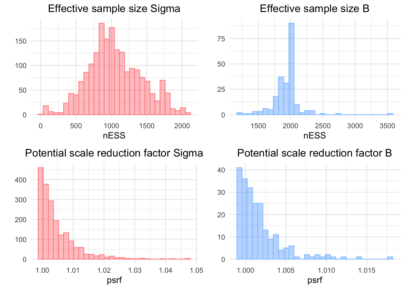
Effective sample size (top panel) and potential scale reduction factor (bot-tom panel) for the correlation matrix Sigma (left panel) and the regression coefficientsB (rigth panel).
Explanatory power of the model
We analyze how well the model can predict the observed data by computing RMSE,TSS and AUC on the observed data.
#Compute predicted values
preds = computePredictedValues(m)
#Compute RMSE and AUC
MF = evaluateModelFit(hM=m, predY=preds)

#Compute TSS
post_mean_preds = data.frame(apply(preds,c(1,2), mean))

TSS = vector()
for (i in 1:nsp){
                  e = evaluate(p=post_mean_preds[which(Y[,i]==1),i], a=post_mean_preds[which(Y[,i]==0),i])
                  index=which.max(e@TPR+e@TNR-1)
                  TSS[i]=e@TPR[index]+e@TNR[index]-1
}
##Cross validation and predictive power of the model We compute the same metrics of above (RMSE,TSS,AUC) in a 2-fold cross validation, to analyze how well the model can predict on data that he was not fitted on.
#Create partition (2 folds)
partition = createPartition(m, nfolds = 2)
#Do cross-validation (2 folds)
preds_espece_CV = computePredictedValues(m, partition = partition,verbose=0)
## Cross-validation, fold 1 out of 2
## Computing chain 1
## Computing chain 2
## Cross-validation, fold 2 out of 2
## Computing chain 1
## Computing chain 2#Compute AUC and RMSE in cross validation
CV = evaluateModelFit(hM = m, predY = preds_espece_CV)
#Compute TSS in cross validation
CV_post_mean_preds = data.frame(apply(preds_espece_CV,c(1,2), mean))
CV_AUC = CV$AUC
TSS_CV = vector()
for (i in 1:nsp){
e = evaluate(p=CV_post_mean_preds[which(Y[,i]==1),i], a=CV_post_mean_preds[which(Y[,i]==0),i])
index=which.max(e@TPR+e@TNR-1)
TSS_CV[i]=e@TPR[index]+e@TNR[index]-1
}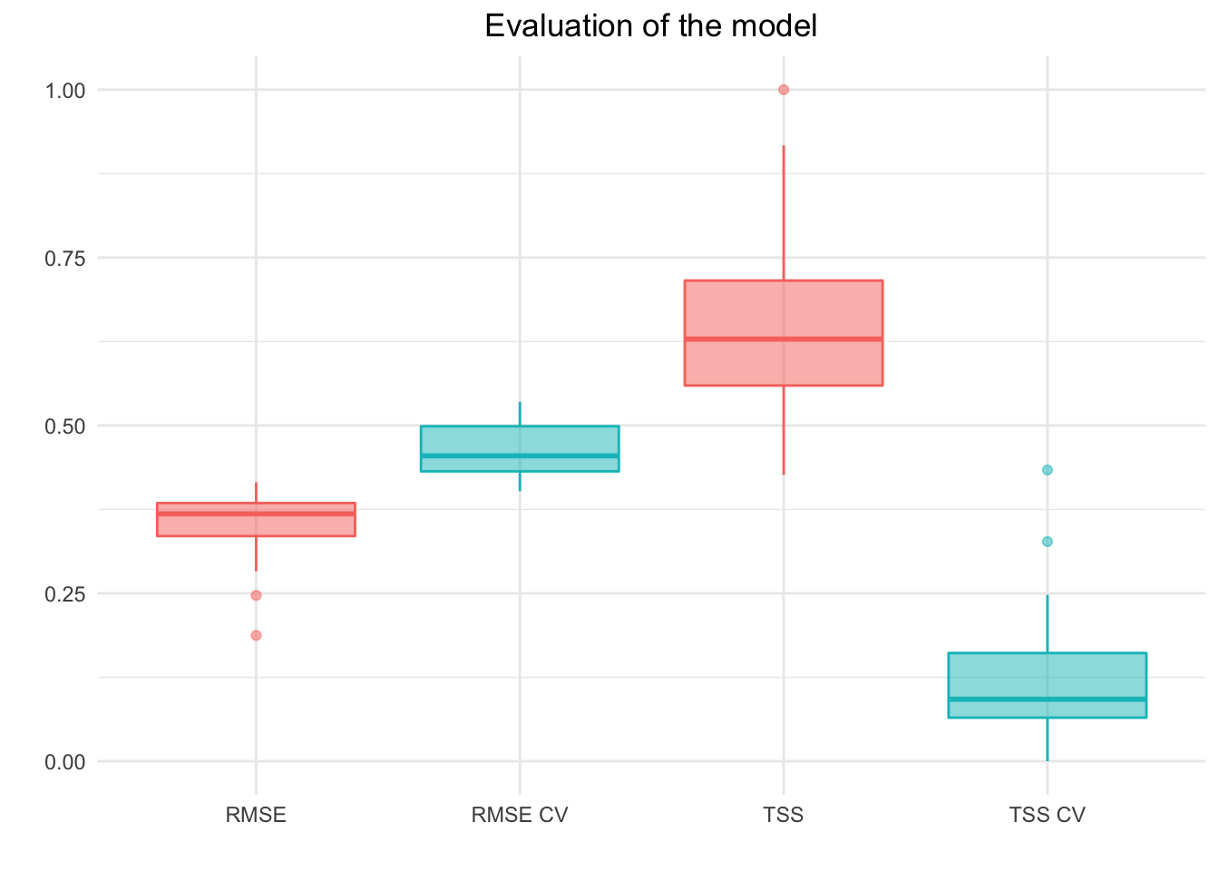
Distribution of TSS and RMSE score across species for in-sample pre-diction (red) and 2-fold cross-validation (blue).
Regression coefficients
We compute and plot here the significant regression coefficients
#Compute regression coefficients
postBeta = getPostEstimate(m, parName="Beta")

#Plot regression coefficients (only those whose 90% credible interval does not overlap zero)
plotBeta(m, post=postBeta, param="Support", supportLevel = 0.9,cex = c(.35,.4,.5),spNamesNumbers = c(T, F),covNamesNumbers = c(F,F))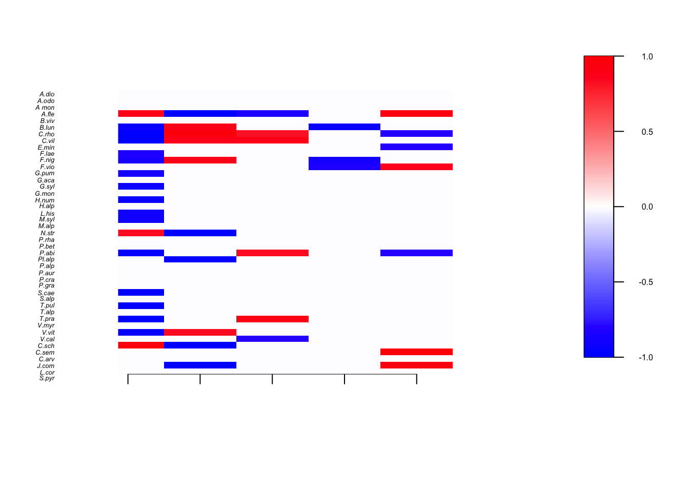
Posterior support values for species regression coefficients. Red if thebounds of the 90% credible interval are both positive, white if the credible interval overlaps 0 and blue if both bounds are negative
Residual correlation matrix
We compute and plot here the significant elements of the residual correlation matrix.
#Compute the residual correlation matrix
OmegaCor = computeAssociations(m)

#Plot residual correlation matrix (only the elements whose 90% credible interval does not overlap zero)
supportLevel = 0.95
toPlot = ((OmegaCor[[1]]$support>supportLevel)
          + (OmegaCor[[1]]$support<(1-supportLevel))>0)*OmegaCor[[1]]$mean

corrplot(toPlot, method = "color", col=colorRampPalette(c("blue","white","red"))(200),
         title=paste("Species associations matrix"), mar=c(0,0,1,0), type="lower",order = "hclust", tl.cex=0.7,diag=F,tl.col = "black")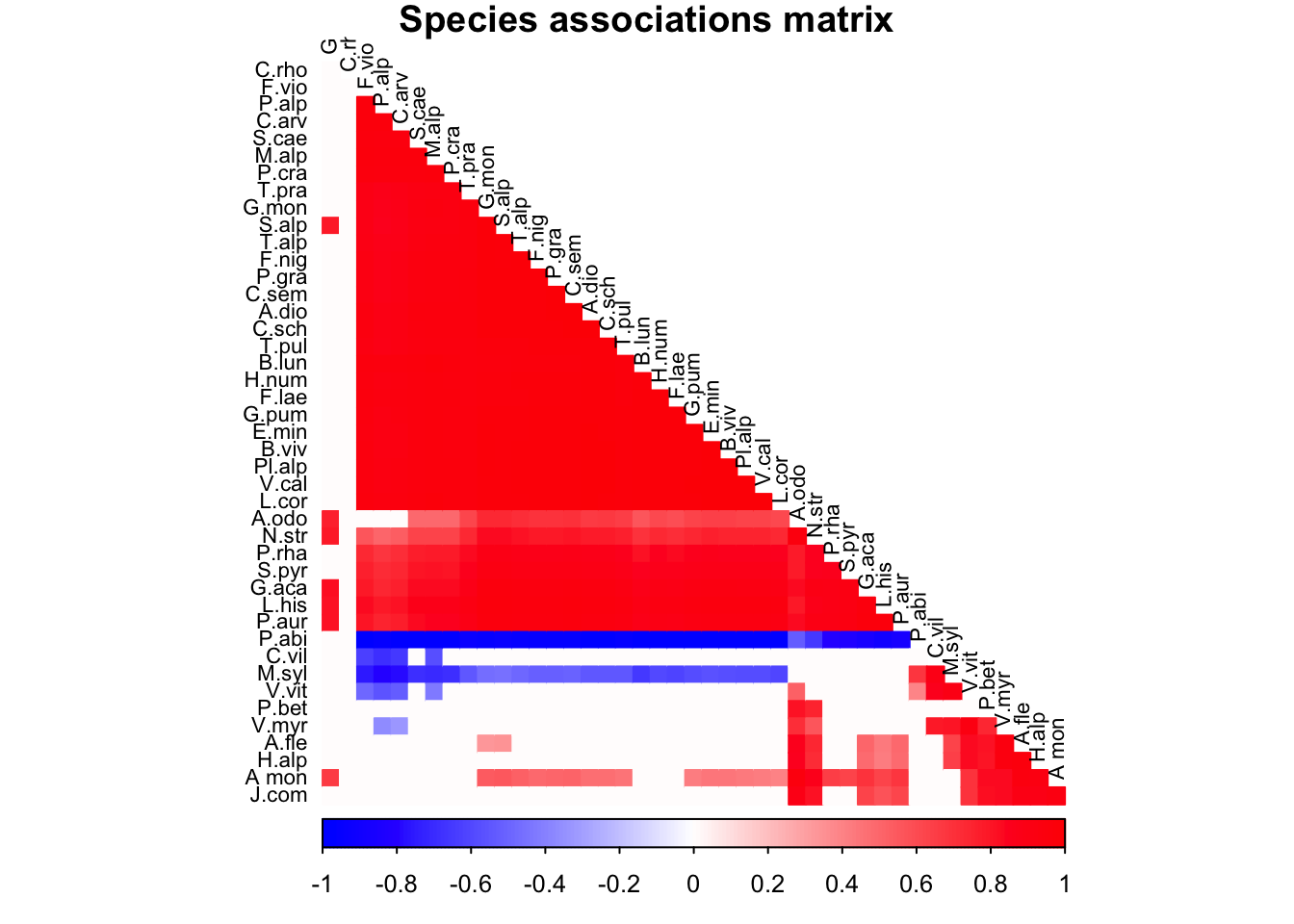
The residual correlation matrix. Only significant values (i.e.95% credible interval do not overlap zero) are shown
Ordination
#Gets the estimates of latent factors and latent loadings
etaPost = getPostEstimate(m, "Eta")
lambdaPost=getPostEstimate(m, "Lambda")

#Biplot
biPlot(m, etaPost = etaPost, lambdaPost=lambdaPost, factors=c(1,2),colors=c("blue","red"))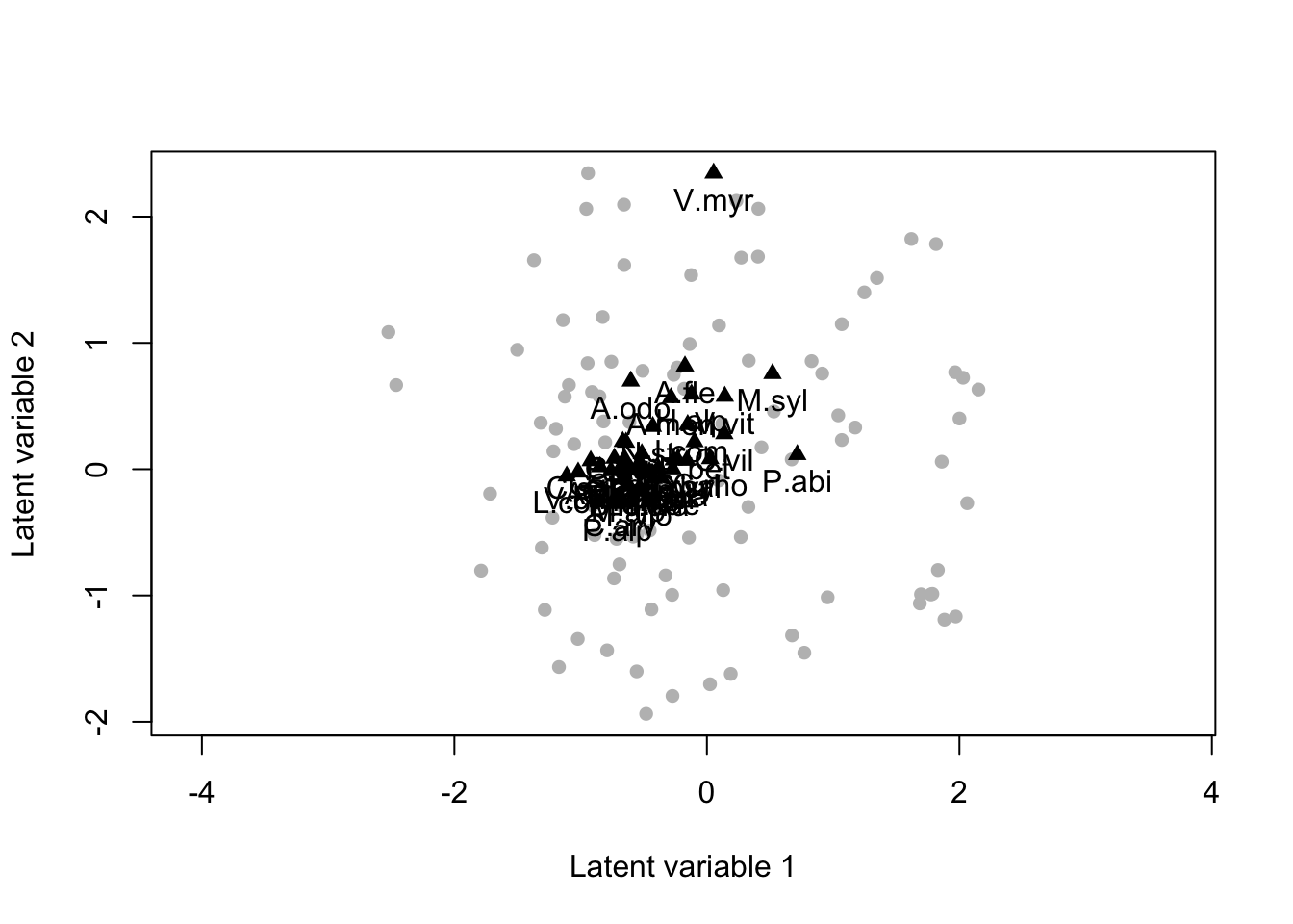
Model based ordination analysis. The two latent variables can be seen as missing covariates, and the position of species (black triangle) on the plot the way species respond to those missing covariates. Species close in the the latent variable species are positively correlated and viceversa.
Include habitat
We now include habitat as a covariate. “Forest” tells us whether a site is forest (“1”) or grassland (“0”). We therefore include such a variable in the matrix of the environmental variable, we re-fit the model, and plot its residual ordination.
# Load environmental data with forest as an additional column (0 if grassland, 1 if forest)
load(file="dat/EnvFor_data.Rdata")

# As above, set model parameters and run the MCMC sampler
studyDesign = data.frame(sample = as.factor(1:nrow(ENV_forest))) #Multivariate random effect
rL = HmscRandomLevel(units = studyDesign$sample)

XFormula=~ENV_forest$pH+ENV_forest$soil_C_N+ENV_forest$Tot_EEA+ENV_forest$GDD.2+ENV_forest$Forest

m_forest = Hmsc(Y = Y, XData = ENV_forest, XFormula = XFormula, studyDesign = studyDesign, ranLevels = list(sample = rL))

thin = 10
samples = 1000
transient = 500
nChains = 2
verbose = 0
m_forest = sampleMcmc(m_forest, thin = thin, samples = samples, transient = transient,
                      nChains = nChains, nParallel = nChains,verbose = verbose)

# Get latent factor and loading
etaPost = getPostEstimate(m_forest, "Eta")
lambdaPost=getPostEstimate(m_forest, "Lambda")

# Plot
biPlot(m_forest, etaPost = etaPost, lambdaPost=lambdaPost, factors=c(1,2))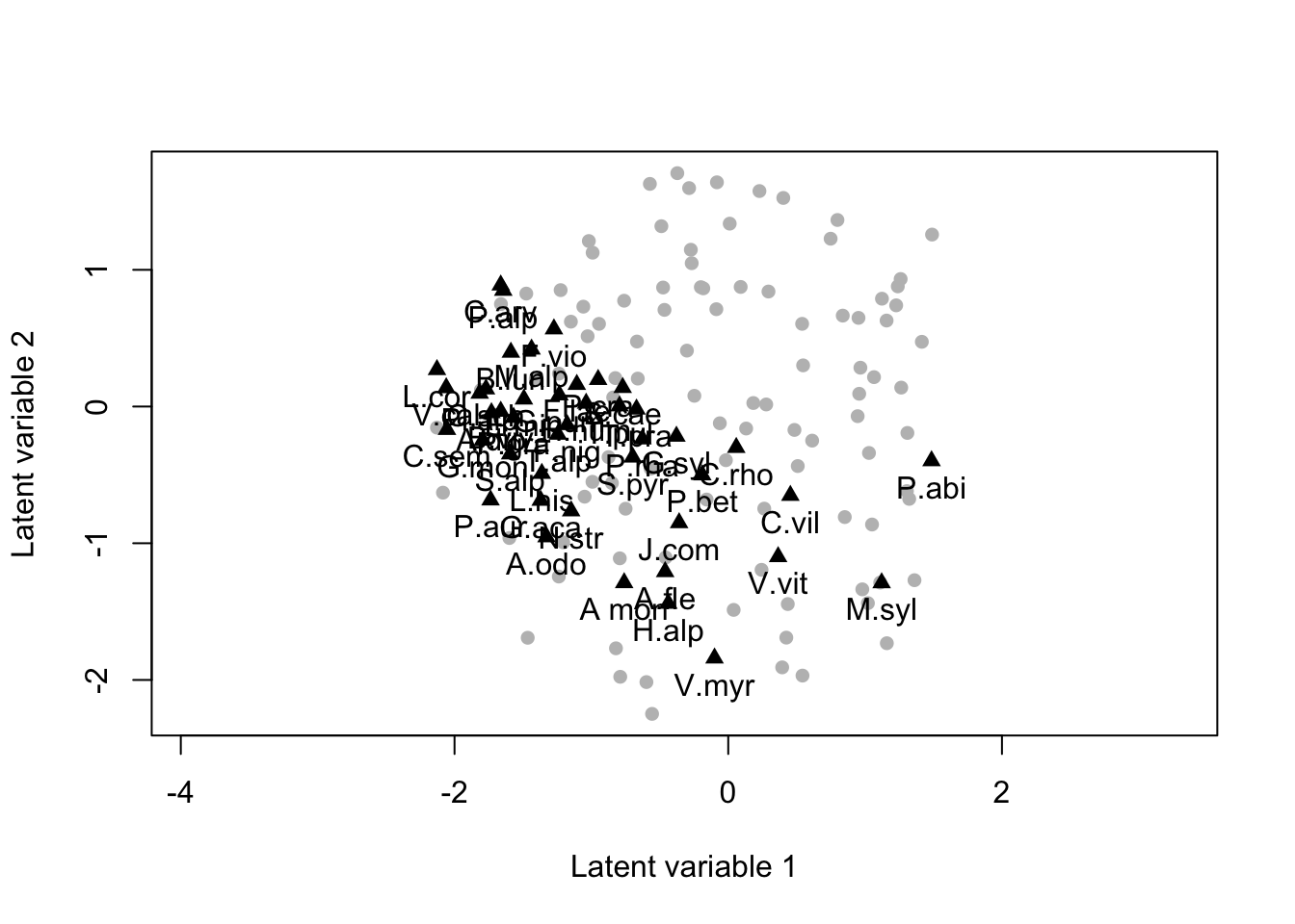
Model based ordination analysis, as above, but when we include the habitat as an additional covariate of the mode.
Conditional prediction in Cross validation
Finally, we compute conditional prediction. Since the prediction ability are more important than the explanotary ones, we compute conditional prediction is Cross Validation (CV).
#Create two folds partition
partition_espece = createPartition(m, nfolds = 2)

#Partition on species, to compute conditional prediction. We condition on Festuca violacea, species number 12
cond_preds_espece_CV_fest = computePredictedValues(m, partition = partition_espece,partition.sp = c(rep(1,times=11),2,rep(1,32)),verbose=0)
## Cross-validation, fold 1 out of 2
## Computing chain 1
## Computing chain 2
## Cross-validation, fold 2 out of 2
## Computing chain 1
## Computing chain 2#Compute AUC and RMSE conditionally on Festuca Violacea, in cross validation
AUC_cond_CV_fest = evaluateModelFit(hM=m, predY=cond_preds_espece_CV_fest)$AUC
#Compute TSS conditionally on Festuca Violacea, in cross validation
mean_cond_preds_espece_CV_fest = data.frame(apply(cond_preds_espece_CV_fest,c(1,2), mean))
TSS_cond_CV_fest = vector()
for (i in 1:nsp){
e = evaluate(p=mean_cond_preds_espece_CV_fest[which(Y[,i]==1),i], a=mean_cond_preds_espece_CV_fest[which(Y[,i]==0),i])
index=which.max(e@TPR+e@TNR-1)
TSS_cond_CV_fest[i]=e@TPR[index]+e@TNR[index]-1
}Predicted probabilities of presence at site Devoluy 21000, conditionally on Festuca violacea and in cross validation
#site choice
site.name="DEV_2100"

#Compute conditional predictions at this site
Cond = data.frame(pred=t(mean_cond_preds_espece_CV_fest[which(rownames(Y)==site.name),]),
                  sp=colnames(Y),type=rep("Conditionally on \n the presence of \n Festuca violacea",nsp),AUC=AUC_cond_CV_fest,presence=Y[rownames(Y)==site.name,])

#Compute unconditional predictions at this site
unCond = data.frame(pred=t(CV_post_mean_preds[which(rownames(Y)==site.name),]),sp=colnames(Y),type=rep("Unconditionally",nsp),AUC=CV_AUC,presence=Y[rownames(Y)==site.name,])
Plot results
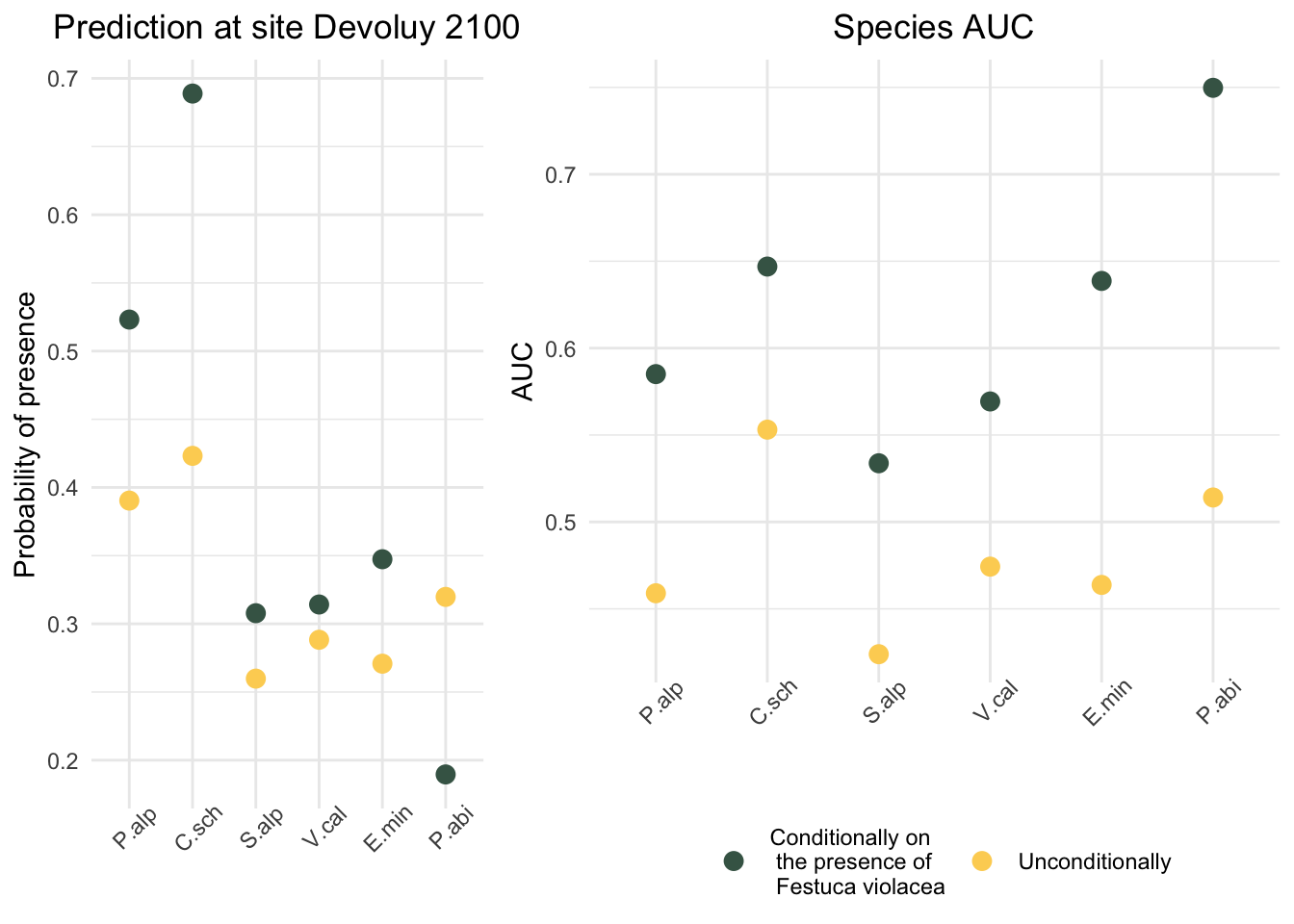
Cross-validation predicted probability of presence (a) and cross-validation AUC (b) of Poa Alpina, Campanula scheuchzeri, Soldanella alpina, Viola calcarata, Euphrasia minima and Picea Abies conditionally on Festuca violacea (green) and unconditionally (yellow). At site Devoluy 2100 all the herbaceous species of above were present (green box) while Picea abies was absent (red box)
References
Martinez-Almoyna, Camille, Gabin Piton, Sylvain Abdulhak, Louise Boulangeat, Philippe Choler, Thierry Delahaye, Cédric Dentant, et al. 2020. “Climate, Soil Resources and Microbial Activity Shape the Distributions of Mountain Plants Based on Their Functional Traits.” Ecography 43 (10): 1550–9. https://doi.org/https://doi.org/10.1111/ecog.05269.
Tikhonov, Gleb, Øystein H. Opedal, Nerea Abrego, Aleksi Lehikoinen, Melinda M. J. de Jonge, Jari Oksanen, and Otso Ovaskainen. 2020. “Joint Species Distribution Modelling with the R-Package Hmsc.” Methods in Ecology and Evolution 11 (3): 442–47. https://doi.org/https://doi.org/10.1111/2041-210X.13345.
Tikhonov, Gleb, Otso Ovaskainen, Jari Oksanen, Melinda de Jonge, Oystein Opedal, and Tad Dallas. 2019. Hmsc: Hierarchical Model of Species Communities. https://CRAN.R-project.org/package=Hmsc.