Inférence de modèles mécanistes en écologie spatiale par une approche mécanistico-statistique
J. Papaïx, L. Roques, S. Soubeyrand, O. Bonnefon, E. Klein, J. Louvrier, E. Walker
Load packages.
library(raster)
library(sp)
library(rgeos)
library(deSolve)
library(Matrix)
library(maptools)
library(unmarked)
library(R2OpenBUGS)
library(coda)
library(plotrix)
Load and format data.
y <- as.matrix(read.table("dat/dony.txt"))
nsite <- ncol(y)
HD_Q <- scan("dat/HD.txt", quiet = T)
forest_Q <- scan("dat/forest.txt",quiet=T)

HD_simuls <- runif(100,min(HD_Q), max(HD_Q))
forest_simuls <- runif(100,min(forest_Q), max(forest_Q))

NsiteOBS <- 100
resolx <- 10
resoly <- 10

# build study area
domaine0 <- rbind(c(-50,-50),c(-50,50),c(50,50),c(50,-50)) # so we can have 28 squares of length 10
r= raster(ncols=resolx,nrows=resoly,ext=extent(min(domaine0[,1]),max(domaine0[,1]),min(domaine0[,2]),max(domaine0[,2])))
domaine <- as(r, 'SpatialPolygons')

# observed sites
coordx = seq(min((domaine0[,1])-(min((domaine0[,1]))/sqrt(NsiteOBS))),
             max((domaine0[,1])-(max((domaine0[,1]))/sqrt(NsiteOBS))), length = sqrt(NsiteOBS))
coordy = seq(min((domaine0[,1])-(min((domaine0[,1]))/sqrt(NsiteOBS))),
             max((domaine0[,1])-(max((domaine0[,1]))/sqrt(NsiteOBS))), length = sqrt(NsiteOBS))

OBSsites <- expand.grid(coordx,coordy)
dataX <- OBSsites[,1]
dataY <- OBSsites[,2]

# get pixel id and area over which we need to integrate
Robs <- (max((domaine0[,1]))/sqrt(NsiteOBS))
OBS <- NULL
for (i in 1:length(dataX)){
  rcenter <-Robs
  coords = matrix(c(dataX[i]-rcenter, dataY[i]-rcenter,
                    dataX[i]-rcenter, dataY[i]+rcenter,
                    dataX[i]+rcenter, dataY[i]+rcenter,
                    dataX[i]+rcenter, dataY[i]-rcenter,
                    dataX[i]-rcenter, dataY[i]-rcenter),
                  ncol = 2, byrow = TRUE)
  P1 = Polygon(coords)
  polyOBS <- list()
  polyOBS[[1]] <- Polygons(list(P1), ID = 1)
  polyOBS <- SpatialPolygons(polyOBS, proj4string= CRS(proj4string(domaine)))
  polyIN <- intersect(polyOBS, domaine)
  areas <- data.frame(area=sapply(polyIN@polygons, FUN=function(x) {slot(x, 'area')}))
  rownames(areas) <- sapply(polyIN@polygons, FUN=function(x) {slot(x, 'ID')})
  numPIX <- as.numeric(matrix(unlist(strsplit(rownames(areas),split=" ")),ncol=2,byrow=T)[,2])
  OBS <- rbind(OBS,cbind(rep(i,length(numPIX)),numPIX,areas$area))
}
colnames(OBS) <- c("OBSsite","SIMsite","area")
plot(domaine)
for (i in 1:length(dataX)){
  rcenter <-Robs
  coords = matrix(c(dataX[i]-rcenter, dataY[i]-rcenter,
                    dataX[i]-rcenter, dataY[i]+rcenter,
                    dataX[i]+rcenter, dataY[i]+rcenter,
                    dataX[i]+rcenter, dataY[i]-rcenter,
                    dataX[i]-rcenter, dataY[i]-rcenter),
                  ncol = 2, byrow = TRUE)
  P1 = Polygon(coords)
  polyOBS <- list()
  polyOBS[[1]] <- Polygons(list(P1), ID = 1)
  polyOBS <- SpatialPolygons(polyOBS, proj4string= CRS(proj4string(domaine)))
  plot(polyOBS, add = T, pch = 24, border = "blue", lwd = 2)
}

points(dataX,dataY,col=2,pch=16,cex=1.5)
plot(domaine, add = T)OBS## OBSsite SIMsite area
## [1,] 1 91 100
## [2,] 2 92 100
## [3,] 3 93 100
## [4,] 4 94 100
## [5,] 5 95 100
## [6,] 6 96 100
## [7,] 7 97 100
## [8,] 8 98 100
## [9,] 9 99 100
## [10,] 10 100 100
## [11,] 11 81 100
## [12,] 12 82 100
## [13,] 13 83 100
## [14,] 14 84 100
## [15,] 15 85 100
## [16,] 16 86 100
## [17,] 17 87 100
## [18,] 18 88 100
## [19,] 19 89 100
## [20,] 20 90 100
## [21,] 21 71 100
## [22,] 22 72 100
## [23,] 23 73 100
## [24,] 24 74 100
## [25,] 25 75 100
## [26,] 26 76 100
## [27,] 27 77 100
## [28,] 28 78 100
## [29,] 29 79 100
## [30,] 30 80 100
## [31,] 31 61 100
## [32,] 32 62 100
## [33,] 33 63 100
## [34,] 34 64 100
## [35,] 35 65 100
## [36,] 36 66 100
## [37,] 37 67 100
## [38,] 38 68 100
## [39,] 39 69 100
## [40,] 40 70 100
## [41,] 41 51 100
## [42,] 42 52 100
## [43,] 43 53 100
## [44,] 44 54 100
## [45,] 45 55 100
## [46,] 46 56 100
## [47,] 47 57 100
## [48,] 48 58 100
## [49,] 49 59 100
## [50,] 50 60 100
## [51,] 51 41 100
## [52,] 52 42 100
## [53,] 53 43 100
## [54,] 54 44 100
## [55,] 55 45 100
## [56,] 56 46 100
## [57,] 57 47 100
## [58,] 58 48 100
## [59,] 59 49 100
## [60,] 60 50 100
## [61,] 61 31 100
## [62,] 62 32 100
## [63,] 63 33 100
## [64,] 64 34 100
## [65,] 65 35 100
## [66,] 66 36 100
## [67,] 67 37 100
## [68,] 68 38 100
## [69,] 69 39 100
## [70,] 70 40 100
## [71,] 71 21 100
## [72,] 72 22 100
## [73,] 73 23 100
## [74,] 74 24 100
## [75,] 75 25 100
## [76,] 76 26 100
## [77,] 77 27 100
## [78,] 78 28 100
## [79,] 79 29 100
## [80,] 80 30 100
## [81,] 81 11 100
## [82,] 82 12 100
## [83,] 83 13 100
## [84,] 84 14 100
## [85,] 85 15 100
## [86,] 86 16 100
## [87,] 87 17 100
## [88,] 88 18 100
## [89,] 89 19 100
## [90,] 90 20 100
## [91,] 91 1 100
## [92,] 92 2 100
## [93,] 93 3 100
## [94,] 94 4 100
## [95,] 95 5 100
## [96,] 96 6 100
## [97,] 97 7 100
## [98,] 98 8 100
## [99,] 99 9 100
## [100,] 100 10 100Function that simulates data from mecastat model.
sim_mecastat <- function(resol_sim, nyear, carrying_capacity, h, intR, betaR, betaRR, intD, betaD, betaDD){

  modLOUP <- function(t,states,parms){
    with(as.list(c(parms,states)),{
      toto <- paste0("U",1:(C*L))
      U <- unlist(mget(toto))
      dU  <- R * U * (1 - U / K) + (alpha * D2 %*% U) / (h * h)
      names(dU)  <- c(paste0("dU", seq(1:(C*L))))
      res <- dU
      list(res)})
  }

  U_matrix <- matrix(0, ncol = resol_sim, nrow = resol_sim)
  C <- ncol(U_matrix)
  L <- nrow(U_matrix)

  # neighboring matrix
  VOIS <- matrix(0,ncol=C*L,nrow=C*L)
  for (i in 1:L){
    for (j in 1:C){
      VOIS.tmp <- matrix(0,ncol=C,nrow=L)
      if((i-1)>=1){VOIS.tmp[i-1,j] <- 1}
      if((i+1)<=L){VOIS.tmp[i+1,j] <- 1}
      if((j-1)>=1){VOIS.tmp[i,j-1] <- 1}
      if((j+1)<=C){VOIS.tmp[i,j+1] <- 1}
      VOIS[(i-1)*C+j,] <- as.vector(t(VOIS.tmp))
    }
  }

  # diffusion if all sites are equal
  M <- diag(-apply(VOIS,1,sum))
  for (i in 1:(C*L)){
    M[i,VOIS[i,]==1] <- 1
  }
  D2 <- M

  # logistic growth rate
  R <- 1 / (1 + exp(-(intR + betaR * forest_simuls + betaRR * forest_simuls^2 )))
  R <- as.vector(t(round(R, digits = 2)))

  # diffusion
  alpha <- 1 / (1 + exp(-(intD + betaD * HD_simuls + betaDD * HD_simuls^2)))

  # parameters
  parms <- c(K = carrying_capacity, R = R, alpha = alpha, h = h, D2 = D2)

  # time
  times <- seq(0, nyear-1, by = 1) # nyears * 12 months

  # first cell(s) to be occupied for initial values
  U_matrix[1,1] <- nb_ind_init
  # initial values
  iniU <- as.vector(t(U_matrix))
  names(iniU) <- c(paste0("U", seq(1:(C*L))))
  inits <- iniU

  # simulations
  simul <- ode(inits, times, modLOUP, parms, method="lsoda")
  list(simul=simul,M=M)
}
Function to fit mecastat wolf model to simulated data (possibly multiple times).
fit_mecastat <- function(resol_fit, nyear, nsurvey, carrying_capacity, intR, betaR, betaRR, intD, betaD, betaDD, detection, nb_ind_init, tol_ode, h, nchains, nburn, niter, debug){

  #-------------------------- simulations ---------------------------- #

  # simulate site-specific abundance - latent states (1)
  run_sim <- sim_mecastat(resol_sim, nyear, carrying_capacity, h, intR, betaR, betaRR, intD, betaD, betaDD)
  simul <- run_sim$simul
  M <- run_sim$M
  L <- C <- resol_fit # squared study area for simplicity here

  # extraction of lambdas
  lambda <- simul[,grep("U",dimnames(simul)[[2]])]

  # simulate counts - latent process (2)
  Ntot <- rpois(length(lambda), lambda) # multipying by 10 the surface of h because
  # so far we were working with a rate but to
  # get a number of individuals per cell
  dim(Ntot) <- dim(lambda)

  # apply detection process - observation process
  # to get the number of times the species has been detected at a site wihin a year,
  r <- detection
  ptemp <- matrix(r, nrow = nyear, ncol = L*C)
  pobs <- 1-(1-ptemp)^Ntot
  nocc <- nb_survey
  nsite <- L*C
  y <- matrix(0, ncol = ncol(pobs), nrow = nrow(pobs))
  for(i in 1:nrow(pobs)){
    for(j in 1:ncol(pobs)){
      y[i,j] <- rbinom(1, nocc, pobs[i,j]) # apply nocc surveys
    }
  }
  y <- t(y)

  #-------------------------- inference ---------------------------- #
  init_onesite <- rep(0, nsite)
  init_onesite[1] <- nb_ind_init

  VOIS <- matrix(0,ncol=C*L,nrow=C*L)
  for (i in 1:L){
    for (j in 1:C){
      VOIS.tmp <- matrix(0,ncol=C,nrow=L)
      if((i-1)>=1){VOIS.tmp[i-1,j] <- 1}
      if((i+1)<=L){VOIS.tmp[i+1,j] <- 1}
      if((j-1)>=1){VOIS.tmp[i,j-1] <- 1}
      if((j+1)<=C){VOIS.tmp[i,j+1] <- 1}
      VOIS[(i-1)*C+j,] <- as.vector(t(VOIS.tmp))
    }
  }

  M <- diag(-apply(VOIS,1,sum))
  for (i in 1:(C*L)){
    M[i,VOIS[i,]==1] <- 1
  }

  # create list of data
  x.data <- list(
    y=y,
    nsite=nsite,
    nyear=nyear,
    v=nocc,
    forest=forest_simuls,
    HD=HD_simuls,
    DD=M,
    h=h,
    origin = 0,
    tol = tol_ode,
    init = init_onesite,
    tgrid = seq(0,nyear-1,by=1))

  # model
  sink("simul_cov_quadra.txt")
  cat("
      model{
      # system of ODEs resolution
      solution[1:nyear, 1:nsite] <- ode(init[1:nsite],
      tgrid[1:nyear],
      D(C[1:nsite], t[nsite]),
      origin,
      tol)
      # abundance model

      for (i in 1:nsite){
      for (j in 1:nsite){
      DDbis[i,j] <- DD[i,j]*alpha1[i]

      }
      }

      for (i in 1:nsite){
      # logistic growth + diffusion
      D(C[i], t[i]) <- rr[i] * C[i] * (1 - C[i] / KK) + inprod(DDbis[i,],C[]) / (h * h)
      logit(rr[i]) <- a.rr + b1.rr * forest[i] + b2.rr * forest[i] * forest[i]
      logit(alpha1[i]) <- a.D + b1.D * HD[i] + b2.D * HD[i] * HD[i]

      }

      for (i in 1:nsite){
      for (k in 1:nyear){
      N[i,k] ~ dpois(solution[k,i])
      }
      }
      # detection model
      for (i in 1:nsite){
      for (k in 1:nyear){
      p[i,k] <- 1 - pow(1 - r, N[i,k])
      y[i,k] ~ dbin(p[i,k],v)
      }
      }

      r ~ dunif(0,1) # detection
      KK ~ dnorm(5,1) # carrying capacity
      a.rr ~ dnorm(0.5,1)T(0,10)
      b1.rr ~ dnorm(0.5,1)T(0,10)
      b2.rr ~ dnorm(0.5,1)T(0,10)
      a.D ~ dnorm(2,1)T(0,10)
      b1.D ~ dnorm(0.5,1)T(0,10)
      b2.D ~ dnorm(0.3,1)T(0,10)

      }
      ")
  sink()

  # specifying the initial MCMC values
  inits <- function()list(
    N = t(Ntot),
    KK = carrying_capacity,
    a.rr = intR,
    b1.rr = betaR,
    b2.rr = betaRR,
    a.D = intD,
    b1.D = betaD,
    b2.D = betaDD,
    r = detection)

  # setting the parameters to be monitored
  params <- c("a.rr","b1.rr","b2.rr","a.D","b1.D","b2.D", "KK","N","r")

  # calling OpenBugs
  OpenBUGS.pgm="C:/Program Files (x86)/OpenBUGS/OpenBUGS323/OpenBUGS.exe"

  ptm <- proc.time()
  wolf.sim <- bugs(x.data, inits, model.file = 'simul_cov_quadra.txt',parameters= params,n.chains = nchains, n.burnin = nburn, n.iter = niter, OpenBUGS.pgm = OpenBUGS.pgm, debug= debug_switch, codaPkg=T)

  elapsed_time = proc.time() - ptm
  elapsed_time
  res <- read.bugs(wolf.sim)

  list(res=res)
}
Simulation study.
resol_sim <- resolx
resol_fit <- resolx
nyear <- 20
carrying_capacity <- 5
intR = 0.4
betaR = 0.4
betaRR = 0.6
intD = 2
betaD = 0.5
betaDD = 0.3
detection <- 0.8
nb_survey <- 4
nb_ind_init <- 1
tol_ode <- 1.0E-3
h <- 10
nchains <- 1
nburn <- 2000
niter <- 10000
debug_switch <- F

# loop on number of simulations
set.seed(13)

H=100
res <- vector("list",H)

estim.median <- matrix(0,nrow=8,ncol=H)
estim.25 <- matrix(0,nrow=8,ncol=H)
estim.975 <- matrix(0,nrow=8,ncol=H)
Run simulations.
for(i in 1:H){

  # estimate parameters of mecastat wolf model
  #res[[i]] <- fit_mecastat(resol_fit, nyear, nsurvey, carrying_capacity, intR, betaR, betaRR, intD, betaD, betaDD, detection, nb_ind_init, tol_ode, h, nchains, nburn, niter, debug_switch)

  estim.median[,i] <- c(median(as.mcmc(res[[i]]$res[,'KK'])), median(as.mcmc(res[[i]]$res[,'a.rr'])),median(as.mcmc(res[[i]]$res[,'b1.rr'])),median(as.mcmc(res[[i]]$res[,'b2.rr'])), median(as.mcmc(res[[i]]$res[,'r'])), median(as.mcmc(res[[i]]$res[,"a.D"])),  median(as.mcmc(res[[i]]$res[,"b1.D"])), median(as.mcmc(res[[i]]$res[,"b2.D"])))
  estim.25[,i]<- c(quantile(as.mcmc(res[[i]]$res[,'KK']),probs=2.5/100),quantile(as.mcmc(res[[i]]$res[,'a.rr']),probs=2.5/100),quantile(as.mcmc(res[[i]]$res[,'b1.rr']),probs=2.5/100),quantile(as.mcmc(res[[i]]$res[,'b2.rr']),probs=2.5/100), quantile(as.mcmc(res[[i]]$res[,'r']),probs=2.5/100),quantile(as.mcmc(res[[i]]$res[,'a.D']),probs=2.5/100), quantile(as.mcmc(res[[i]]$res[,'b1.D']),probs=2.5/100), quantile(as.mcmc(res[[i]]$res[,'b2.D']),probs=2.5/100))
  estim.975[,i] <- c(quantile(as.mcmc(res[[i]]$res[,'KK']),probs=97.5/100),quantile(as.mcmc(res[[i]]$res[,'a.rr']),probs=97.5/100),quantile(as.mcmc(res[[i]]$res[,'b1.rr']),probs=97.5/100),quantile(as.mcmc(res[[i]]$res[,'b2.rr']),probs=97.5/100), quantile(as.mcmc(res[[i]]$res[,'r']),probs=97.5/100),quantile(as.mcmc(res[[i]]$res[,'a.D']),probs=97.5/100), quantile(as.mcmc(res[[i]]$res[,'b1.D']),probs=97.5/100), quantile(as.mcmc(res[[i]]$res[,'b2.D']),probs=97.5/100))

  print(i)
}

save(res, estim.median, estim.25, estim.975, file = 'resHPHR_covs2_quadra_10000it_prior_inf4.RData')
Use this link to download the results (file of size 100Mo approx).
load("dat/resHPHR_covs2_quadra_10000it_prior_inf4.RData")Check out convergence.
par(mfrow = c(4,2))

i=2

plot(as.vector(as.mcmc(res[[1]]$res[,'KK'])), type = "l", ylim = c(0,10), main = "KK")
lines(as.vector(as.mcmc(res[[i]]$res[,'KK'])), col = "green" )

plot(as.vector(as.mcmc(res[[1]]$res[,'a.rr'])), type = "l", ylim = c(0,1), main = "a.rr")
lines(as.vector(as.mcmc(res[[i]]$res[,'a.rr'])), col = "green")

plot(as.vector(as.mcmc(res[[1]]$res[,'b1.rr'])), type = "l", ylim = c(0,2), main = "b1.rr")
lines(as.vector(as.mcmc(res[[i]]$res[,'b1.rr'])), col = "green")

plot(as.vector(as.mcmc(res[[1]]$res[,'b2.rr'])), type = "l", ylim = c(0,2), main = "b2.rr")
lines(as.vector(as.mcmc(res[[i]]$res[,'b2.rr'])), col = "green")

plot(as.vector(as.mcmc(res[[1]]$res[,'r'])), type = "l", ylim = c(0,1), main = "r")
lines(as.vector(as.mcmc(res[[i]]$res[,'r'])), col = "green")

plot(as.vector(as.mcmc(res[[1]]$res[,'a.D'])), type = "l", ylim = c(0,10), main = "a.D")
lines(as.vector(as.mcmc(res[[i]]$res[,'a.D'])), col = "green")

plot(as.vector(as.mcmc(res[[1]]$res[,'b1.D'])), type = "l", ylim = c(0,10), main = "b1.D")
lines(as.vector(as.mcmc(res[[i]]$res[,'b1.D'])), col = "green")

plot(as.vector(as.mcmc(res[[1]]$res[,'b2.D'])), type = "l", ylim = c(0,10), main = "b2.D")
lines(as.vector(as.mcmc(res[[i]]$res[,'b2.D'])), col = "green")
Posterior densities.
plot(density(as.mcmc(res[[1]]$res[,'KK'])), type = "l", ylim = c(0,1), main = "KK, prior = dunif(0,25)",xlim = c(-1,10))
lines(density(as.mcmc(res[[2]]$res[,'KK'])), col = "green")
curve(dnorm(x,5,1), col = "blue", add =T)
abline(v = 5, col = "red")
legend("topright", c("chain1", "chain2", "prior"," true value"), col = c("black","green","blue","red"), lwd = 1)

plot(density(as.mcmc(res[[1]]$res[,'a.rr'])), type = "l", ylim = c(0,2), main = "a.rr, prior = dlnorm(1,1)", xlim = c(-1,3))
lines(density(as.mcmc(res[[i]]$res[,'a.rr'])), col = "green")
curve(dnorm(x,0.5,1), col = "blue", add =T)
abline(v = 0.4, col = "red")
legend("topright", c("chain1", "chain2", "prior"," true value"), col = c("black","green","blue","red"), lwd = 1)

plot(density(as.mcmc(res[[1]]$res[,'b1.rr'])), type = "l", ylim = c(0,2), main = "b1.rr, prior = dunif(0,10)", xlim = c(-1,4))
lines(density(as.mcmc(res[[i]]$res[,'b1.rr'])), col = "green")
curve(dnorm(x,0.5,1), col = "blue", add =T)
abline(v = 0.4, col = "red")
legend("topright", c("chain1", "chain2", "prior"," true value"), col = c("black","green","blue","red"), lwd = 1)

plot(density(as.mcmc(res[[1]]$res[,'b2.rr'])), type = "l", ylim = c(0,1.5), main = "b2.rr, prior = dunif(0,10)", xlim = c(-1,2))
lines(density(as.mcmc(res[[i]]$res[,'b2.rr'])), col = "green")
curve(dnorm(x,0.5,1), col = "blue", add =T)
abline(v = 0.6, col = "red")
legend("topright", c("chain1", "chain2", "prior"," true value"), col = c("black","green","blue","red"), lwd = 1)

plot(density(as.mcmc(res[[1]]$res[,'r'])), type = "l", ylim = c(0,12), main = "r, prior = dunif(0,1)", xlim = c(-0.5,1.5))
lines(density(as.mcmc(res[[i]]$res[,'r'])), col = "green")
curve(dunif(x,0,1), col = "blue", add =T)
abline(v = 0.2, col = "red")
legend("topright", c("chain1", "chain2", "prior"," true value"), col = c("black","green","blue","red"), lwd = 1)

plot(density(as.mcmc(res[[1]]$res[,'a.D'])), type = "l", ylim = c(0,1.5), main = "a.D, prior = dlnorm(1,1)")
lines(density(as.mcmc(res[[i]]$res[,'a.D'])), col = "green")
curve(dnorm(x,2,1), col = "blue", add =T)
abline(v = 2, col = "red")
legend("topright", c("chain1", "chain2", "prior"," true value"), col = c("black","green","blue","red"), lwd = 1)

plot(density(as.mcmc(res[[1]]$res[,'b1.D'])), type = "l", ylim = c(0,1), main = "b1.D, prior = dunif(0,10)")
lines(density(as.mcmc(res[[i]]$res[,'b1.D'])), col = "green")
curve(dnorm(x,0.5,1), col = "blue", add =T)
abline(v = 0.5, col = "red")
legend("topright", c("chain1", "chain2", "prior"," true value"), col = c("black","green","blue","red"), lwd = 1)

plot(density(as.mcmc(res[[1]]$res[,'b2.D'])), type = "l", ylim = c(0,1), main = "b2.D, prior = dunif(0,10)", xlim = c(-1,11))
lines(density(as.mcmc(res[[i]]$res[,'b2.D'])), col = "green")
curve(dnorm(x,0.3,1), col = "blue", add =T)
abline(v = 0.3, col = "red")
legend("topright", c("chain1", "chain2", "prior"," true value"), col = c("black","green","blue","red"), lwd = 1)
Compute bias and MSE.
H <- 100
Bias <- matrix(0,nrow=1, ncol = 8)
MSE <- matrix(0,nrow=1, ncol = 8)
x <- matrix(0, nrow = H, ncol =8)
diff <- matrix(0, nrow = H, ncol = 8)
param <- c(carrying_capacity, intR, betaR, betaRR, detection, intD, betaD, betaDD)

#K
for(i in 1:H){
  x[i,1] <- mean(as.mcmc(res[[i]]$res[,'KK']))
  diff[i,1] <- (x[i,1]-param[1])
}

#rr
for(i in 1:H){
  x[i,2] <- mean(as.mcmc(res[[i]]$res[,'a.rr']))
  diff[i,2] <- (x[i,2]-param[2])
}

#b1.rr
for(i in 1:H){
  x[i,3] <- mean(as.mcmc(res[[i]]$res[,'b1.rr']))
  diff[i,3] <- (x[i,3]-param[3])
}

#r
for(i in 1:H){
  x[i,4] <- mean(as.mcmc(res[[i]]$res[,'b2.rr']))
  diff[i,4] <- (x[i,4]-param[4])
}

#r
for(i in 1:H){
  x[i,5] <- mean(as.mcmc(res[[i]]$res[,'r']))
  diff[i,5] <- (x[i,5]-param[5])
}

#a.D
for(i in 1:H){
  x[i,6] <- mean(as.mcmc(res[[i]]$res[,'a.D']))
  diff[i,6] <- (x[i,6]-param[6])
}

#b1.D
for(i in 1:H){
  x[i,7] <- mean(as.mcmc(res[[i]]$res[,'b1.D']))
  diff[i,7] <- (x[i,7]-param[7])
}

#b2.D
for(i in 1:H){
  x[i,8] <- mean(as.mcmc(res[[i]]$res[,'b2.D']))
  diff[i,8] <- (x[i,8]-param[8])
}

for(i in 1:length(param)) {
  Bias[i] <- ((mean(x[,i])-param[i])/param[i])*100
  MSE[i] <- mean((diff[,i])^2)
}
Bias
## [,1] [,2] [,3] [,4] [,5] [,6] [,7] [,8]
## [1,] 1.579092 10.64683 33.38791 12.84218 -1.025791 3.672924 89.27693 196.8127MSE## [,1] [,2] [,3] [,4] [,5] [,6]
## [1,] 0.2176843 0.02207432 0.06204329 0.04529993 0.001404637 0.06391005
## [,7] [,8]
## [1,] 0.2166324 0.3737464Visualise bias and MSE.
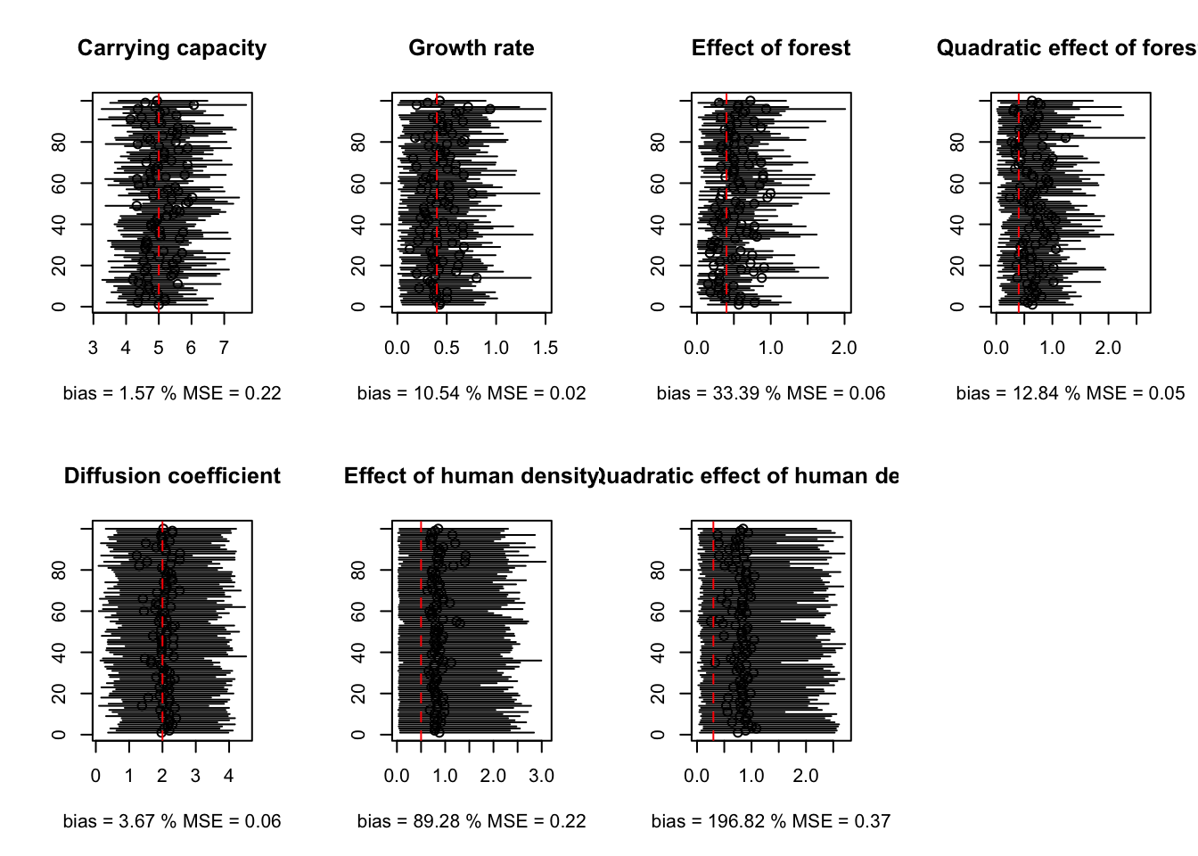
par(mfrow=c(2,4))

plot(estim.median[1,], 1:H, ylab='',xlim=range(c(estim.median[1,],estim.25[1,],estim.975[1,])),main='Carrying capacity', xlab = 'bias = 1.57 % MSE = 0.22')
segments(estim.25[1,], 1:H, estim.975[1,], 1:100)
abline(v=carrying_capacity, lty=2, col='red')


plot(estim.median[2,], 1:H, ylab='',xlim=range(c(estim.median[2,],estim.25[2,],estim.975[2,])),main='Growth rate', xlab = 'bias = 10.54 % MSE = 0.02')
segments(estim.25[2,], 1:H, estim.975[2,], 1:100)
abline(v=intR, lty=2, col='red')


plot(estim.median[3,], 1:H, ylab='',xlim=range(c(estim.median[3,],estim.25[3,],estim.975[3,])),main='Effect of forest', xlab = 'bias = 33.39 % MSE = 0.06')
segments(estim.25[3,], 1:H, estim.975[3,], 1:100)
abline(v=betaR, lty=2, col='red')

plot(estim.median[4,], 1:H, ylab='',xlim=range(c(estim.median[4,],estim.25[4,],estim.975[4,])),main='Quadratic effect of forest', xlab = 'bias = 12.84 % MSE = 0.05')
segments(estim.25[4,], 1:H, estim.975[4,], 1:100)
abline(v=betaR, lty=2, col='red')

plot(estim.median[6,], 1:H, ylab='',xlim=range(c(estim.median[6,],estim.25[6,],estim.975[6,])),main='Diffusion coefficient', xlab = 'bias = 3.67 % MSE = 0.06')
segments(estim.25[6,], 1:H, estim.975[6,], 1:100)
abline(v=intD, lty=2, col='red')

plot(estim.median[7,], 1:H, ylab='',xlim=range(c(estim.median[7,],estim.25[7,],estim.975[7,])),main='Effect of human density', xlab = 'bias = 89.28 % MSE = 0.22')
segments(estim.25[7,], 1:H, estim.975[7,], 1:100)
abline(v=betaD, lty=2, col='red')

plot(estim.median[8,], 1:H, ylab='',xlim=range(c(estim.median[8,],estim.25[8,],estim.975[8,])),main='Quadratic effect of human density', xlab = 'bias = 196.82 % MSE = 0.37')
segments(estim.25[8,], 1:H, estim.975[8,], 1:100)
abline(v=betaDD, lty=2, col='red')