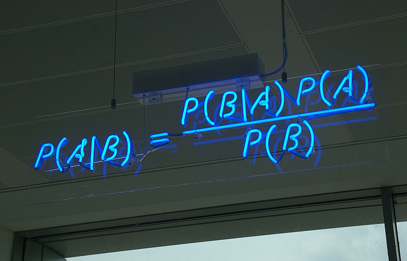
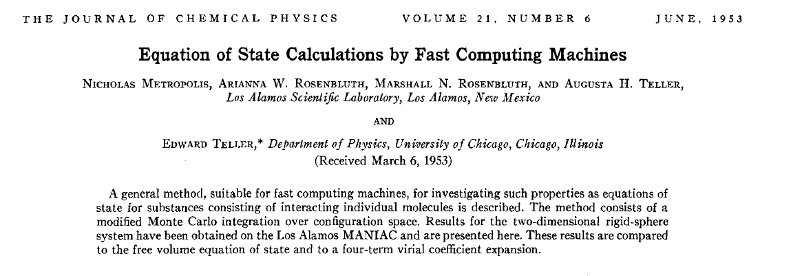
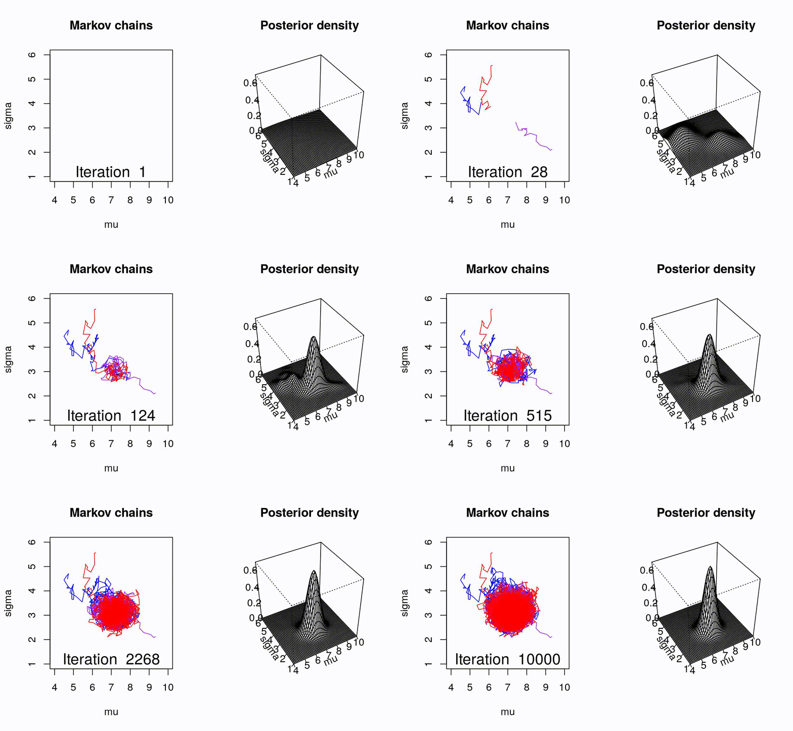
class: center, middle, title-slide .title[ # Crash course on Bayesian statistics and MCMC algorithms ] .date[ ### last updated: 2023-07-01 ] --- class: center, middle background-image: url(img/amazing-thomas-bayes-illustration.jpg) background-size: cover --- # Bayes' theorem .pull-left[ .title-font[] * A theorem about conditional probabilities. * `\(\Pr(B \mid A) = \displaystyle{\frac{ \Pr(A \mid B) \; \Pr(B)}{\Pr(A)}}\)` ] .pull-right[ .title-font[] .center[  ] .tiny[Bayes' theorem spelt out in blue neon at the offices of Autonomy in Cambridge. Source: Wikipedia] ] --- # Bayes' theorem + I always forget what the letters mean. -- + Might be easier to remember when written like this: $$ \Pr(\text{hypothesis} \mid \text{data}) = \frac{ \Pr(\text{data} \mid \text{hypothesis}) \; \Pr(\text{hypothesis})}{\Pr(\text{data})} $$ -- + The "hypothesis" is typically something unobserved or unknown. It's what you want to learn about using the data. -- + For regression models, the "hypothesis" is a parameter (intercept, slopes or error terms). -- + Bayes theorem tells you the probability of the hypothesis given the data. --- # What is doing science after all? <br> <br> -- How plausible is some hypothesis given the data? $$ \Pr(\text{hypothesis} \mid \text{data}) = \frac{ \Pr(\text{data} \mid \text{hypothesis}) \; \Pr(\text{hypothesis})}{\Pr(\text{data})} $$ ??? + The Bayesian reasoning echoes the scientific reasoning. + You might ask then, why is Bayesian statistics not the default? --- # Why is Bayesian statistics not the default? -- + Due to practical problems of implementing the Bayesian approach, and futile wars between (male) statisticians, little progress was made for over two centuries. -- + Recent advances in computational power coupled with the development of new methodology have led to a great increase in the application of Bayesian methods within the last two decades. --- # Frequentist versus Bayesian -- + Typical stats problems involve estimating parameter `\(\theta\)` with available data. -- + The frequentist approach (maximum likelihood estimation – MLE) assumes that the parameters are fixed, but have unknown values to be estimated. -- + Classical estimates are generally point estimates of the parameters of interest. -- + The Bayesian approach assumes that the parameters are not fixed but have some fixed unknown distribution - a distribution for the parameter. --- # What is the Bayesian approach? -- + The approach is based upon the idea that the experimenter begins with some prior beliefs about the system. ??? + You never start from scratch. -- + And then updates these beliefs on the basis of observed data. -- + This updating procedure is based upon the Bayes' Theorem: `$$\Pr(A \mid B) = \frac{\Pr(B \mid A) \; \Pr(A)}{\Pr(B)}$$` --- # What is the Bayesian approach? -- + Schematically if `\(A = \theta\)` and `\(B = \text{data}\)`, then -- + The Bayes' theorem `$$\Pr(A \mid B) = \frac{\Pr(B \mid A) \; \Pr(A)}{\Pr(B)}$$` -- + Translates into: `$$\Pr(\theta \mid \text{data}) = \frac{\Pr(\text{data} \mid \theta) \; \Pr(\theta)}{\Pr(\text{data})}$$` --- # Bayes' theorem `$${\color{red}{\Pr(\theta \mid \text{data})}} = \frac{\color{blue}{\Pr(\text{data} \mid \theta)} \; \color{green}{\Pr(\theta)}}{\color{orange}{\Pr(\text{data})}}$$` -- + `\(\color{red}{\text{Posterior distribution}}\)`: Represents what you know after having seen the data. The basis for inference, a distribution, possibly multivariate if more than one parameter. -- + `\(\color{blue}{\text{Likelihood}}\)`: This quantity is the same as in the MLE approach. -- + `\(\color{green}{\text{Prior distribution}}\)`: Represents what you know before seeing the data. The source of much discussion about the Bayesian approach. -- + `\(\color{orange}{\Pr(\text{data}) = \int{L(\text{data} \mid \theta)\Pr(\theta) d\theta}}\)` is a `\(N\)`-dimensional integral if `\(\theta = \theta_1, \ldots, \theta_N\)`. -- + Difficult if not impossible to calculate. This is one of the reasons why we need simulation (MCMC) methods. --- # Brute force via numerical integration -- + Say we release `\(n\)` animals at the beginning of the winter, out of which `\(y\)` survive, and we'd like to estimate winter survival `\(\theta\)`. ```r y <- 19 # nb of success n <- 57 # nb of attempts ``` -- + Our model: `\begin{align*} y &\sim \text{Binomial}(n, \theta) &\text{[likelihood]} \\ \theta &\sim \text{Beta}(1, 1) &\text{[prior for }\theta \text{]} \\ \end{align*}` --- # Beta prior .center.nogap[ <!-- --> ] --- # Apply Bayes theorem + Likelihood times the prior: `\(\Pr(\text{data} \mid \theta) \; \Pr(\theta)\)` ```r numerator <- function(p) dbinom(y,n,p) * dbeta(p,a,b) ``` + Averaged likelihood: `\(\Pr(\text{data}) = \int{L(\theta \mid \text{data}) \; \Pr(\theta) d\theta}\)` ```r denominator <- integrate(numerator,0,1)$value ``` --- # Posterior via numerical integration .center.nogap[ <!-- --> ] --- # Superimpose explicit posterior .center.nogap[ <!-- --> ] --- # And the prior .center.nogap[ <!-- --> ] --- # What if multiple parameters? + Example of a linear regression with parameters `\(\alpha\)`, `\(\beta\)` and `\(\sigma\)` to be estimated. -- + Bayes' theorem says: $$ P(\alpha, \beta, \sigma \mid \text{data}) = \frac{ P(\text{data} \mid \alpha, \beta, \sigma) \, P(\alpha, \beta, \sigma)}{\iiint \, P(\text{data} \mid \alpha, \beta, \sigma) \, P(\alpha, \beta, \sigma) \,d\alpha \,d\beta \,d\sigma} $$ -- + Do we really wish to calculate a 3D integral? --- # Bayesian computation -- + In the early 1990s, statisticians rediscovered work from the 1950's in physics. .center[  ] --- # Bayesian computation + In the early 1990s, statisticians rediscovered work from the 1950's in physics. -- + Use stochastic simulation to draw samples from posterior distributions. -- + Avoid explicit calculation of integrals in Bayes formula. -- + Instead, approx. posterior w/ some precision by drawing large samples. -- * Markov chain Monte Carlo (MCMC) gives a boost to Bayesian statistics! --- class: center, middle background-image: url(img/maniac1.png) background-size: cover --- class: center, middle background-image: url(img/maniac2.png) background-size: cover --- # Why are MCMC methods so useful? -- + MCMC are stochastic algorithms to produce sequence of dependent random numbers from a Markov chain. -- + A Markov chain is a discrete sequence of states, in which the probability of an event depends only on the state in the previous event. -- + A Markov chain has an equilibrium (aka stationary) distribution. -- + Equilibrium distribution is the desired posterior distribution! -- + Several ways of constructing these chains: e.g., Metropolis-Hastings, Gibbs sampler. -- + How to implement them in practice?! --- # The Metropolis algorithm -- + Let's go back to animal survival estimation. -- + We illustrate sampling from the posterior distribution. -- + We write functions in `R` for the likelihood, the prior and the posterior. --- ```r # survival data, 19 "success" out of 57 "attempts" survived <- 19 released <- 57 # log-likelihood function loglikelihood <- function(x, p){ dbinom(x = x, size = released, prob = p, log = TRUE) } # prior density logprior <- function(p){ dunif(x = p, min = 0, max = 1, log = TRUE) } # posterior density function (log scale) posterior <- function(x, p){ loglikelihood(x, p) + logprior(p) # - log(Pr(data)) } ``` --- ## Metropolis algorithm -- 1. We start at any possible value of the parameter to be estimated. -- 2. To decide where to visit next, we propose to move away from the current value of the parameter <span>&#8212;</span> this is a **candidate** value. To do so, we add to the current value some random value from say a normal distribution with some variance. -- 3. We compute the ratio of the probabilities at the candidate and current locations `\(R = \text{posterior(candidate)/posterior(current)}\)`. This is where the magic of MCMC happens, in that `\(\Pr(\text{data})\)`, the denominator of the Bayes theorem, cancels out. -- 4. We spin a continuous spinner that lands anywhere from 0 to 1 <span>&#8212;</span> call it the random spin `\(X\)`. If `\(X\)` is smaller than `\(R\)`, we move to the candidate location, otherwise we remain at the current location. -- 5. We repeat 2-4 a number of times <span>&#8212;</span> or **steps** (many steps). --- ```r # propose candidate value move <- function(x, away = .2){ logitx <- log(x / (1 - x)) logit_candidate <- logitx + rnorm(1, 0, away) candidate <- plogis(logit_candidate) return(candidate) } # set up the scene steps <- 100 theta.post <- rep(NA, steps) set.seed(1234) # pick starting value (step 1) inits <- 0.5 theta.post[1] <- inits ``` --- ```r for (t in 2:steps){ # repeat steps 2-4 (step 5) # propose candidate value for prob of success (step 2) theta_star <- move(theta.post[t-1]) # calculate ratio R (step 3) pstar <- posterior(survived, p = theta_star) pprev <- posterior(survived, p = theta.post[t-1]) logR <- pstar - pprev R <- exp(logR) # decide to accept candidate value or to keep current value (step 4) accept <- rbinom(1, 1, prob = min(R, 1)) theta.post[t] <- ifelse(accept == 1, theta_star, theta.post[t-1]) } ``` --- Starting at the value `\(0.5\)` and running the algorithm for `\(100\)` iterations. ```r head(theta.post) ``` ``` [1] 0.5000000 0.4399381 0.4399381 0.4577124 0.4577124 0.4577124 ``` ```r tail(theta.post) ``` ``` [1] 0.4145878 0.3772087 0.3772087 0.3860516 0.3898536 0.3624450 ``` --- ## A chain .center.nogap[ <!-- --> ] --- ## Another chain .center.nogap[ <!-- --> ] --- ## With 5000 steps .center.nogap[ <!-- --> ] In yellow: posterior mean; in red: maximum likelihood estimate. --- ### Animating MCMC - 1D example (code [here](https://gist.github.com/oliviergimenez/5ee33af9c8d947b72a39ed1764040bf3)) .center[ ] --- background-color: #FCFCFF ### Animating MCMC - 2D example (code [here](https://mbjoseph.github.io/posts/2018-12-25-animating-the-metropolis-algorithm/)) .center[  ] --- ## The MCMC Interactive Gallery (more [here](https://chi-feng.github.io/mcmc-demo/)) .center[  ] --- # Assessing convergence -- + MCMC algorithms can be used to construct a Markov chain with a given stationary distribution (set to be the posterior distribution). -- + For the MCMC algorithm, the posterior distribution is only needed to be known up to proportionality. -- + Once the stationary distribution is reached, we can regard the realisations of the chain as a (dependent) sample from the posterior distribution (and obtain Monte Carlo estimates). -- + We consider some important implementation issues. --- ## Mixing and autocorrelation .center.nogap[ <!-- --> ] ??? + The movement around the parameter space is often referred to as **mixing**. + Traceplots of for small and big moves provide (relatively) high correlations (known as autocorrelations) between successive observations of the Markov chain. + Strongly correlated observations require large sample sizes and therefore longer simulations. + Autocorrelation function (ACF) plots are a convenient way of displaying the strength of autocorrelation in the given sample values. + ACF plots provide the autocorrelation between successively sampled values separated by `\(k\)` iterations, referred to as lag, (i.e. `\(\text{cor}(\theta_t, \theta_{t+k})\)`) for increasing values of `\(k\)`. --- # How do good chains behave? -- + Converge to same target distribution; discard some realisations of Markov chain before convergence is achieved. -- + Once there, explore efficiently: The post-convergence sample size required for suitable numerical summaries. -- + Therefore, we are looking to determine how long it takes for the Markov chain to converge to the stationary distribution. -- + In practice, we must discard observations from the start of the chain and just use observations from the chain once it has converged. -- + The initial observations that we discard are referred to as the **burn-in**. -- + Simplest method to determine length of burn-in period is to look at trace plots. --- ## Burn-in .center.nogap[ <!-- --> ] If simulations cheap, be conservative. --- # Effective sample size `n.eff` -- * How long of a chain is needed to produce stable estimates ? -- * Most MCMC chains are strongly autocorrelated. -- * Successive steps are near each other, and are not independent. -- * The effective sample size (`n.eff`) measures chain length while taking into account the autocorrelation of the chain. * `n.eff` is less than the number of MCMC iterations. * Check the `n.eff` of every parameter of interest. * Check the `n.eff` of any interesting parameter combinations. -- * We need `\(\text{n.eff} \geq 100\)` independent steps. --- # Potential scale reduction factor -- + Gelman-Rubin statistic `\(\hat{R}\)` -- + Measures the ratio of the total variability combining multiple chains (between-chain plus within-chain) to the within-chain variability. -- + Asks the question is there a chain effect? Very much alike the `\(F\)` test in an ANOVA. -- + Values near `\(1\)` indicates likely convergence, a value of `\(\leq 1.1\)` is considered acceptable. -- + Necessary condition, not sufficient; In other words, these diagnostics cannot tell you that you have converged for sure, only that you have not. --- # To sum up -- + Run multiple chains from arbitrary starting places (initial values). -- + Assume convergence when all chains reach same regime -- + Discard initial burn-in phase. -- + Proceed with posterior inference. -- + Use traceplot, effective sample size and `\(\hat{R}\)`. --- # What if you have issues of convergence? -- + Increase burn-in, sample more. -- + Use more informative priors. -- + Pick better initial values (good guess), using e.g. estimates from simpler models. -- + Reparameterize: + Standardize covariates. + Non-centering: `\(\alpha \sim N(0,\sigma)\)` becomes `\(\alpha = z \sigma\)` with `\(z \sim N(0,1)\)`. -- + Something wrong with your model? + Start with a simpler model (remove complexities). + Use simulations. -- + Change your sampler. More later on. --- # Further reading + McCarthy, M. (2007). [Bayesian Methods for Ecology](https://www.cambridge.org/core/books/bayesian-methods-for-ecology/9225F65B8A25D69B0B6C50B5A9A78201). Cambridge: Cambridge University Press. + McElreath, R. (2020). [Statistical Rethinking: A Bayesian Course with Examples in R and Stan (2nd ed.)](https://xcelab.net/rm/statistical-rethinking/). CRC Press. + Gelman, A. and Hill, J. (2006). [Data Analysis Using Regression and Multilevel/Hierarchical Models (Analytical Methods for Social Research)](https://www.cambridge.org/core/books/data-analysis-using-regression-and-multilevelhierarchical-models/32A29531C7FD730C3A68951A17C9D983). Cambridge: Cambridge University Press. --- background-color: #234f66 ## <span style="color:white">Live demo</span> .center[  ]